INSTRUCTORS Carleen Eaton Grant Fraser Eric Smith

Eric Smith

Eric Smith

Graphing Functions

Slide Duration:

Table of Contents

Section 1: Properties of Real Numbers
Basic Types of Numbers

30m 41s

Intro
0:00
Objectives
0:07
Basic Types of Numbers
0:36
Natural Numbers
1:02
Whole Numbers
1:29
Integers
2:04
Rational Numbers
2:38
Irrational Numbers
5:06
Imaginary Numbers
6:48
Basic Types of Numbers Cont.
8:09
The Big Picture
8:10
Real vs. Imaginary Numbers
8:30
Rational vs. Irrational Numbers
8:48
Basic Types of Numbers Cont.
10:55
Number Line
11:06
Absolute Value
11:44
Inequalities
12:39
Example 1
13:16
Example 2
17:30
Example 3
21:56
Example 4
24:27
Example 5
27:48
Operations on Numbers

19m 26s

Intro
0:00
Objectives
0:06
Operations on Numbers
0:25
Addition
0:53
Subtraction
1:33
Multiplication & Division
2:19
Exponents
3:24
Bases
4:04
Square Roots
4:59
Principle Square Roots
5:09
Perfect Squares
6:32
Simplifying and Combining Roots
6:52
Example 1
8:16
Example 2
12:30
Example 3
14:02
Example 4
16:27
Order of Operations

12m 6s

Intro
0:00
Objectives
0:06
The Order of Operations
0:25
Work Inside Parentheses
0:42
Simplify Exponents
0:52
Multiplication & Division from Left to Right
0:57
Addition & Subtraction from Left to Right
1:11
Remember PEMDAS
1:21
The Order of Operations Cont.
2:27
Example
2:43
Example 1
3:55
Example 2
5:36
Example 3
7:35
Example 4
8:56
Properties of Real Numbers

18m 52s

Intro
0:00
Objectives
0:07
The Properties of Real Numbers
0:23
Commutative Property of Addition and Multiplication
0:44
Associative Property of Addition and Multiplication
1:50
Distributive Property of Multiplication Over Addition
3:20
Division Property of Zero
4:46
Division Property of One
5:23
Multiplication Property of Zero
5:56
Multiplication Property of One
6:17
Addition Property of Zero
6:29
Why Are These Properties Important?
6:53
Example 1
9:16
Example 2
13:04
Example 3
14:30
Example 4
16:57
Section 2: Linear Equations
The Vocabulary of Linear Equations

12m 22s

Intro
0:00
Objectives
0:09
The Vocabulary of Linear Equations
0:44
Variables
0:52
Terms
1:09
Coefficients
1:40
Like Terms
2:18
Examples of Like Terms
2:37
Expressions
4:01
Equations
4:26
Linear Equations
5:04
Solutions
5:55
Example 1
6:16
Example 2
7:16
Example 3
8:45
Example 4
10:20
Solving Linear Equations in One Variable

28m 52s

Intro
0:00
Objectives
0:08
Solving Linear Equations in One Variable
0:34
Conditional Cases
0:51
Identity Cases
1:09
Contradiction Cases
1:30
Solving Linear Equations in One Variable Cont.
2:00
Addition Property of Equality
2:10
Multiplication Property of Equality
2:43
Steps to Solve Linear Equations
3:14
Example 1
4:22
Example 2
8:21
Example 3
12:32
Example 4
14:19
Example 5
17:25
Example 6
22:17
Solving Formulas

12m 2s

Intro
0:00
Objectives
0:06
Solving Formulas
0:18
Formulas
0:26
Use the Same Properties as Solving Linear Equations
1:36
Addition Property of Equality
1:55
Multiplication Property of Equality
1:58
Steps to Solve Formulas
2:43
Example 1
3:56
Example 2
6:09
Example 3
8:39
Applications of Linear Equations

28m 41s

Intro
0:00
Objectives
0:10
Applications of Linear Equations
0:43
The Six-Step Method to Solving Word Problems
0:55
Common Terms
3:12
Example 1
5:03
Example 2
9:40
Example 3
13:48
Example 4
17:58
Example 5
23:28
Applications of Linear Equations, Motion & Mixtures

24m 26s

Intro
0:00
Objectives
0:21
Motion and Mixtures
0:46
Motion Problems: Distance, Rate, and Time
1:06
Mixture Problems: Amount, Percent, and Total
1:27
The Table Method
1:58
The Beaker Method
3:38
Example 1
5:05
Example 2
9:44
Example 3
14:20
Example 4
19:13
Section 3: Graphing
Rectangular Coordinate System

22m 55s

Intro
0:00
Objectives
0:11
The Rectangular Coordinate System
0:39
The Cartesian Coordinate System
0:40
X-Axis
0:54
Y-Axis
1:04
Origin
1:11
Quadrants
1:26
Ordered Pairs
2:10
Example 1
2:55
The Rectangular Coordinate System Cont.
6:09
X-Intercept
6:45
Y-Intercept
6:55
Relation of X-Values and Y-Values
7:30
Example 2
11:03
Example 3
12:13
Example 4
14:10
Example 5
18:38
Slope & Graphing

27m 58s

Intro
0:00
Objectives
0:11
Slope and Graphing
0:48
Standard Form
1:14
Example 1
2:24
Slope and Graphing Cont.
4:58
Slope, m
5:07
Slope is Rise over Run
6:11
Don't Mix Up the Coordinates
8:20
Example 2
9:39
Slope and Graphing Cont.
14:26
Slope-Intercept Form
14:34
Example 3
16:55
Example 4
18:00
Slope and Graphing Cont.
19:00
Rewriting an Equation in Slope-Intercept Form
19:39
Rewriting an Equation in Standard Form
20:09
Slopes of Vertical & Horizontal Lines
20:56
Example 5
22:49
Example 6
24:09
Example 7
25:59
Example 8
26:57
Linear Equations in Two Variables

20m 36s

Intro
0:00
Objectives
0:13
Linear Equations in Two Variables
0:36
Point-Slope Form
1:07
Substitute in the Point and the Slope
2:21
Parallel Lines: Two Lines with the Same Slope
4:05
Perpendicular Lines: Slopes are Negative Reciprocals of Each Other
4:39
Perpendicular Lines: Product of Slopes is -1
5:24
Example 1
6:02
Example 2
7:50
Example 3
10:49
Example 4
13:26
Example 5
15:30
Example 6
17:43
Section 4: Functions
Introduction to Functions

21m 24s

Intro
0:00
Objectives
0:07
Introduction to Functions
0:58
Relations
1:03
Functions
1:37
Independent Variables
2:00
Dependent Variables
2:11
Function Notation
2:21
Function
3:43
Input and Output
3:53
Introduction to Functions Cont.
4:45
Domain
4:46
Range
4:55
Functions Represented by a Diagram
6:41
Natural Domain
9:11
Evaluating Functions
12:02
Example 1
13:13
Example 2
15:03
Example 3
16:18
Example 4
19:54
Graphing Functions

16m 12s

Intro
0:00
Objectives
0:09
Graphing Functions
0:54
Using Slope-Intercept Form
1:56
Vertical Line Test
2:58
Determining the Domain
4:20
Determining the Range
5:43
Example 1
6:06
Example 2
7:18
Example 3
8:31
Example 4
11:04
Section 5: Systems of Linear Equations
Systems of Linear Equations

25m 54s

Intro
0:00
Objectives
0:13
Systems of Linear Equations
0:46
System of Equations
0:51
System of Linear Equations
1:15
Solutions
1:35
Points as Solutions
1:53
Finding Solutions Graphically
5:13
Example 1
6:37
Example 2
12:07
Systems of Linear Equations Cont.
17:01
One Solution, No Solution, or Infinite Solutions
17:10
Example 3
18:31
Example 4
22:37
Solving a System Using Substitution

20m 1s

Intro
0:00
Objectives
0:09
Solving a System Using Substitution
0:32
Substitution Method
1:24
Substitution Example
2:35
One Solution, No Solution, or Infinite Solutions
7:50
Example 1
9:45
Example 2
12:48
Example 3
15:01
Example 4
17:30
Solving a System Using Elimination

19m 40s

Intro
0:00
Objectives
0:09
Solving a System Using Elimination
0:27
Elimination Method
0:42
Elimination Example
2:01
One Solution, No Solution, or Infinite Solutions
7:05
Example 1
8:53
Example 2
11:46
Example 3
15:37
Example 4
17:45
Applications of Systems of Equations

24m 34s

Intro
0:00
Objectives
0:12
Applications of Systems of Equations
0:30
Word Problems
1:31
Example 1
2:17
Example 2
7:55
Example 3
13:07
Example 4
17:15
Section 6: Inequalities
Solving Linear Inequalities in One Variable

17m 13s

Intro
0:00
Objectives
0:08
Solving Linear Inequalities in One Variable
0:37
Inequality Expressions
0:46
Linear Inequality Solution Notations
3:40
Inequalities
3:51
Interval Notation
4:04
Number Lines
4:43
Set Builder Notation
5:24
Use Same Techniques as Solving Equations
6:59
'Flip' the Sign when Multiplying or Dividing by a Negative Number
7:12
'Flip' Example
7:50
Example 1
8:54
Example 2
11:40
Example 3
14:01
Compound Inequalities

16m 13s

Intro
0:00
Objectives
0:07
Compound Inequalities
0:37
'And' vs. 'Or'
0:44
'And'
3:24
'Or'
3:35
'And' Symbol, or Intersection
3:51
'Or' Symbol, or Union
4:13
Inequalities
4:41
Example 1
6:22
Example 2
9:30
Example 3
11:27
Example 4
13:49
Solving Equations with Absolute Values

14m 12s

Intro
0:00
Objectives
0:08
Solve Equations with Absolute Values
0:18
Solve Equations with Absolute Values Cont.
1:11
Steps to Solving Equations with Absolute Values
2:21
Example 1
3:23
Example 2
6:34
Example 3
10:12
Inequalities with Absolute Values

17m 7s

Intro
0:00
Objectives
0:07
Inequalities with Absolute Values
0:23
Recall…
2:08
Example 1
3:39
Example 2
6:06
Example 3
8:14
Example 4
10:29
Example 5
13:29
Graphing Inequalities in Two Variables

15m 33s

Intro
0:00
Objectives
0:07
Graphing Inequalities in Two Variables
0:32
Split Graph into Two Regions
1:53
Graphing Inequalities
5:44
Test Points
6:20
Example 1
7:11
Example 2
10:17
Example 3
13:06
Systems of Inequalities

21m 13s

Intro
0:00
Objectives
0:08
Systems of Inequalities
0:24
Test Points
1:10
Steps to Solve Systems of Inequalities
1:25
Example 1
2:23
Example 2
7:28
Example 3
12:51
Section 7: Polynomials
Integer Exponents

44m 51s

Intro
0:00
Objectives
0:09
Integer Exponents
0:42
Exponents 'Package' Multiplication
1:25
Example 1
2:00
Example 2
3:13
Integer Exponents Cont.
4:50
Product Rule for Exponents
4:51
Example 3
7:16
Example 4
10:15
Integer Exponents Cont.
13:13
Power Rule for Exponents
13:14
Power Rule with Multiplication and Division
15:33
Example 5
16:18
Integer Exponents Cont.
20:04
Example 6
20:41
Integer Exponents Cont.
25:52
Zero Exponent Rule
25:53
Quotient Rule
28:24
Negative Exponents
30:14
Negative Exponent Rule
32:27
Example 7
34:05
Example 8
36:15
Example 9
39:33
Example 10
43:16
Adding & Subtracting Polynomials

18m 33s

Intro
0:00
Objectives
0:07
Adding and Subtracting Polynomials
0:25
Terms
0:33
Coefficients
0:51
Leading Coefficients
1:13
Like Terms
1:29
Polynomials
2:21
Monomials, Binomials, Trinomials, and Polynomials
5:41
Degrees
7:00
Evaluating Polynomials
8:12
Adding and Subtracting Polynomials Cont.
9:25
Example 1
11:48
Example 2
13:00
Example 3
14:41
Example 4
16:15
Multiplying Polynomials

25m 7s

Intro
0:00
Objectives
0:06
Multiplying Polynomials
0:41
Distributive Property
1:00
Example 1
2:49
Multiplying Polynomials Cont.
8:22
Organize Terms with a Table
8:23
Example 2
13:40
Multiplying Polynomials Cont.
16:33
Multiplying Binomials with FOIL
16:48
Example 3
18:49
Example 4
20:04
Example 5
21:42
Dividing Polynomials

44m 56s

Intro
0:00
Objectives
0:07
Dividing Polynomials
0:29
Dividing Polynomials by Monomials
2:10
Dividing Polynomials by Polynomials
2:59
Dividing Numbers
4:09
Dividing Polynomials Example
8:39
Example 1
12:35
Example 2
14:40
Example 3
16:45
Example 4
21:13
Example 5
24:33
Example 6
29:02
Dividing Polynomials with Synthetic Division Method
33:36
Example 7
38:43
Example 8
42:24
Section 8: Factoring Polynomials
Greatest Common Factor & Factor by Grouping

28m 27s

Intro
0:00
Objectives
0:09
Greatest Common Factor
0:31
Factoring
0:40
Greatest Common Factor (GCF)
1:48
GCF for Polynomials
3:28
Factoring Polynomials
6:45
Prime
8:21
Example 1
9:14
Factor by Grouping
14:30
Steps to Factor by Grouping
17:03
Example 2
17:43
Example 3
19:20
Example 4
20:41
Example 5
22:29
Example 6
26:11
Factoring Trinomials

21m 44s

Intro
0:00
Objectives
0:06
Factoring Trinomials
0:25
Recall FOIL
0:26
Factor a Trinomial by Reversing FOIL
1:52
Tips when Using Reverse FOIL
5:31
Example 1
7:04
Example 2
9:09
Example 3
11:15
Example 4
13:41
Factoring Trinomials Cont.
15:50
Example 5
18:42
Factoring Trinomials Using the AC Method

30m 9s

Intro
0:00
Objectives
0:08
Factoring Trinomials Using the AC Method
0:27
Factoring when Leading Term has Coefficient Other Than 1
1:07
Reversing FOIL
1:18
Example 1
1:46
Example 2
4:28
Factoring Trinomials Using the AC Method Cont.
7:45
The AC Method
8:03
Steps to Using the AC Method
8:19
Tips on Using the AC Method
9:29
Example 3
10:45
Example 4
16:50
Example 5
21:08
Example 6
24:58
Special Factoring Techniques

30m 14s

Intro
0:00
Objectives
0:07
Special Factoring Techniques
0:26
Difference of Squares
1:46
Perfect Square Trinomials
2:38
No Sum of Squares
3:32
Special Factoring Techniques Cont.
4:03
Difference of Squares Example
4:04
Perfect Square Trinomials Example
5:29
Example 1
7:31
Example 2
9:59
Example 3
11:47
Example 4
15:09
Special Factoring Techniques Cont.
19:07
Sum of Cubes and Difference of Cubes
19:08
Example 5
23:13
Example 6
26:12
Section 9: Quadratic Equations
Solving Quadratic Equations by Factoring

23m 38s

Intro
0:00
Objectives
0:08
Solving Quadratic Equations by Factoring
0:19
Quadratic Equations
0:20
Zero Factor Property
1:39
Zero Factor Property Example
2:34
Example 1
4:00
Solving Quadratic Equations by Factoring Cont.
5:54
Example 2
7:28
Example 3
11:09
Example 4
14:22
Solving Quadratic Equations by Factoring Cont.
18:17
Higher Degree Polynomial Equations
18:18
Example 5
20:22
Solving Quadratic Equations

29m 27s

Intro
0:00
Objectives
0:12
Solving Quadratic Equations
0:29
Linear Factors
0:38
Not All Quadratics Factor Easily
1:22
Principle of Square Roots
3:36
Completing the Square
4:50
Steps for Using Completing the Square
5:15
Completing the Square Works on All Quadratic Equations
6:41
The Quadratic Formula
7:28
Discriminants
8:25
Solving Quadratic Equations - Summary
10:11
Example 1
11:54
Example 2
13:03
Example 3
16:30
Example 4
21:29
Example 5
25:07
Equations in Quadratic Form

16m 47s

Intro
0:00
Objectives
0:08
Equations in Quadratic Form
0:24
Using a Substitution
0:53
U-Substitution
1:26
Example 1
2:07
Example 2
5:36
Example 3
8:31
Example 4
11:14
Quadratic Formulas & Applications

29m 4s

Intro
0:00
Objectives
0:09
Quadratic Formulas and Applications
0:35
Squared Variable
0:40
Principle of Square Roots
0:51
Example 1
1:09
Example 2
2:04
Quadratic Formulas and Applications Cont.
3:34
Example 3
4:42
Example 4
13:33
Example 5
20:50
Graphs of Quadratics

26m 53s

Intro
0:00
Objectives
0:06
Graphs of Quadratics
0:39
Axis of Symmetry
1:46
Vertex
2:12
Transformations
2:57
Graphing in Quadratic Standard Form
3:23
Example 1
5:06
Example 2
6:02
Example 3
9:07
Graphs of Quadratics Cont.
11:26
Completing the Square
12:02
Vertex Shortcut
12:16
Example 4
13:49
Example 5
17:25
Example 6
20:07
Example 7
23:43
Polynomial Inequalities

21m 42s

Intro
0:00
Objectives
0:07
Polynomial Inequalities
0:30
Solving Polynomial Inequalities
1:20
Example 1
2:45
Polynomial Inequalities Cont.
5:12
Larger Polynomials
5:13
Positive or Negative Intervals
7:16
Example 2
9:01
Example 3
13:53
Section 10: Rational Equations
Multiply & Divide Rational Expressions

26m 41s

Intro
0:00
Objectives
0:09
Multiply and Divide Rational Expressions
0:44
Rational Numbers
0:55
Dividing by Zero
1:45
Canceling Extra Factors
2:43
Negative Signs in Fractions
4:52
Multiplying Fractions
6:26
Dividing Fractions
7:17
Example 1
8:04
Example 2
14:01
Example 3
16:23
Example 4
18:56
Example 5
22:43
Adding & Subtracting Rational Expressions

20m 24s

Intro
0:00
Objectives
0:07
Adding and Subtracting Rational Expressions
0:41
Common Denominators
0:52
Common Denominator Examples
1:14
Steps to Adding and Subtracting Rational Expressions
2:39
Example 1
3:34
Example 2
5:27
Adding and Subtracting Rational Expressions Cont.
6:57
Least Common Denominators
6:58
Transitioning from Fractions to Rational Expressions
9:08
Identifying Least Common Denominators for Rational Expressions
9:56
Subtracting vs. Adding
10:41
Example 3
11:19
Example 4
12:36
Example 5
15:08
Example 6
16:46
Complex Fractions

18m 23s

Intro
0:00
Objectives
0:09
Complex Fractions
0:37
Dividing to Simplify Complex Fractions
1:10
Example 1
2:03
Example 2
3:58
Complex Fractions Cont.
9:15
Using the Least Common Denominator to Simplify Complex Fractions
9:16
Both Methods Lead to the Same Answer
10:07
Example 3
10:42
Example 4
14:28
Solving Rational Equations

16m 24s

Intro
0:00
Objectives
0:07
Solving Rational Equations
0:23
Isolate the Specified Variable
1:23
Example 1
1:58
Example 2
5:00
Example 3
8:23
Example 4
13:25
Rational Inequalities

18m 54s

Intro
0:00
Objectives
0:06
Rational Inequalities
0:18
Testing Intervals for Rational Inequalities
0:38
Steps to Solving Rational Inequalities
1:05
Tips to Solving Rational Inequalities
2:27
Example 1
3:33
Example 2
12:21
Applications of Rational Expressions

20m 20s

Intro
0:00
Objectives
0:07
Applications of Rational Expressions
0:27
Work Problems
1:05
Example 1
2:58
Example 2
6:45
Example 3
13:17
Example 4
16:37
Variation & Proportion

27m 4s

Intro
0:00
Objectives
0:10
Variation and Proportion
0:34
Variation
0:35
Inverse Variation
1:01
Direct Variation
1:10
Setting Up Proportions
1:31
Example 1
2:27
Example 2
5:36
Variation and Proportion Cont.
8:29
Inverse Variation
8:30
Example 3
9:20
Variation and Proportion Cont.
12:41
Constant of Proportionality
12:42
Example 4
13:59
Variation and Proportion Cont.
16:17
Varies Directly as the nth Power
16:30
Varies Inversely as the nth Power
16:53
Varies Jointly
17:09
Combining Variation Models
17:36
Example 5
19:09
Example 6
22:10
Section 11: Radical Equations
Rational Exponents

14m 32s

Intro
0:00
Objectives
0:07
Rational Exponents
0:32
Power on Top, Root on Bottom
1:05
Example 1
1:37
Rational Exponents Cont.
4:04
Using Rules from Exponents for Radicals as Exponents
4:05
Combining Terms Under a Single Root
4:50
Example 2
5:21
Example 3
7:39
Example 4
11:23
Example 5
13:14
Simplify Rational Exponents

15m 12s

Intro
0:00
Objectives
0:07
Simplify Rational Exponents
0:25
Product Rule for Radicals
0:26
Product Rule to Simplify Square Roots
1:11
Quotient Rule for Radicals
1:42
Applications of Product and Quotient Rules
2:17
Higher Roots
2:48
Example 1
3:39
Example 2
6:35
Example 3
8:41
Example 4
11:09
Adding & Subtracting Radicals

17m 22s

Intro
0:00
Objectives
0:07
Adding and Subtracting Radicals
0:33
Like Terms
1:29
Bases and Exponents May be Different
2:02
Bases and Powers Must be Same when Adding and Subtracting
2:42
Add Radicals' Coefficients
3:55
Example 1
4:47
Example 2
6:00
Adding and Subtracting Radicals Cont.
7:10
Simplify the Bases to Look the Same
7:25
Example 3
8:23
Example 4
11:45
Example 5
15:10
Multiply & Divide Radicals

19m 24s

Intro
0:00
Objectives
0:08
Multiply and Divide Radicals
0:25
Rules for Working With Radicals
0:26
Using FOIL for Radicals
1:11
Don’t Distribute Powers
2:54
Dividing Radical Expressions
4:25
Rationalizing Denominators
6:40
Example 1
7:22
Example 2
8:32
Multiply and Divide Radicals Cont.
9:23
Rationalizing Denominators with Higher Roots
9:25
Example 3
10:51
Example 4
11:53
Multiply and Divide Radicals Cont.
13:13
Rationalizing Denominators with Conjugates
13:14
Example 5
15:52
Example 6
17:25
Solving Radical Equations

15m 5s

Intro
0:00
Objectives
0:07
Solving Radical Equations
0:17
Radical Equations
0:18
Isolate the Roots and Raise to Power
0:34
Example 1
1:13
Example 2
3:09
Solving Radical Equations Cont.
7:04
Solving Radical Equations with More than One Radical
7:05
Example 3
7:54
Example 4
13:07
Complex Numbers

29m 16s

Intro
0:00
Objectives
0:06
Complex Numbers
1:05
Imaginary Numbers
1:08
Complex Numbers
2:27
Real Parts
2:48
Imaginary Parts
2:51
Commutative, Associative, and Distributive Properties
3:35
Adding and Subtracting Complex Numbers
4:04
Multiplying Complex Numbers
6:16
Dividing Complex Numbers
8:59
Complex Conjugate
9:07
Simplifying Powers of i
14:34
Shortcut for Simplifying Powers of i
18:33
Example 1
21:14
Example 2
22:15
Example 3
23:38
Example 4
26:33
Loading...
This is a quick preview of the lesson. For full access, please Log In or Sign up.
For more information, please see full course syllabus of Algebra 1
Bookmark & Share Embed

Share this knowledge with your friends!

Copy & Paste this embed code into your website’s HTML

Please ensure that your website editor is in text mode when you paste the code.
(In Wordpress, the mode button is on the top right corner.)
  ×
  • - Allow users to view the embedded video in full-size.
Since this lesson is not free, only the preview will appear on your website.
  • Discussion

  • Answer Engine

  • Study Guides

  • Practice Questions

  • Download Lecture Slides

  • Table of Contents

  • Transcription

  • Related Books

Lecture Comments (4)

1 answer

Last reply by: Educator Study
Sat May 20, 2023 2:04 PM

Post by Educator Study on May 20, 2023

You're shit.

1 answer

Last reply by: Professor Eric Smith
Tue Apr 22, 2014 8:33 PM

Post by Wanda Thomas on April 1, 2014

Hello Professor,

Enjoying your lectures. Glad I found this site to assist with my preparation for a CLEP exam.

I have some questions.
Will you please expound on when the rule for using y2 or y1 for the y factor? I notice some problems use on or the other.

Also, please the answer to this problem:
. A line passes through the points (5, - 4) and ( - 1,6). Find the equation of this line in slope intercept form.

*These practice questions are only helpful when you work on them offline on a piece of paper and then use the solution steps function to check your answer.

   Step 1. m = [(y2 − y1)/(x2 − x1)]
   Step 2. m = [(6 − ( − 4))/( − 1 − 5)]
   Step 3. m = − [10/6] = − [5/3]
   Step 4. 6 = − [5/3]( − 1) + b
   Step 5. 6 = 1[2/3] + b

Answer
4[1/3] = b   ***Where did the 4 come from?***

Graphing Functions

  • We can graph functions using a table of values. This is the same process that is used for graphing equations.
  • To create a table of values, choose several values for the independent variable, then evaluate the function for these values. This will develop of a list of ordered pairs (inputs, outputs) that can be plotted.
  • You can determine if a graph is a function by using the vertical line test. If the graph crosses a vertical line in more than one spot, it is not a function.
  • To determine the domain and range of a function from its graph, trace points back to the x-axis and y-axis. The points traced back to the x-axis will cover the domain. The points traced back to the y-axis will cover the range.

Graphing Functions

A line passes through the points (5,4) and (0,8). Find the equation of the line in slope intercept form.
  • y = mx + b
    slope = [(y2 − y1)/(x2 − x1)]
  • slope = [(8 − 4)/(0 − 5)] = [4/( − 5)]
y = − [4/5]x + 8
A line passes through the points ( - 3,6) and (0, - 6). Find the equation of the line in slope intercept form.
  • y = mx + b
    slope = [(y2 − y1)/(x2 − x1)]
  • slope = [( − 6 − 6)/(0 − ( − 3))]
  • slope = [( − 12)/3]
  • slope = − 4
y = − 4x − 6
A line has slope - 4 and passes through ( - 10, - 8). Find its equation in slope intercept form.
  • y = mx + b
  • m = − 4
    b = ?
  • − 8 = − 4( − 10) + b
  • − 8 = 40 + b
  • b = − 48
y = − 4x − 48
A line has slope - 1 and passes through (7,15). Find its equation in slope intercept form.
  • y = mx + b
  • m = − 1
    b = ?
  • 15 = − 1(7) + b
  • 15 = − 7 + b
  • 22 = b
  • y = − 1x + 22
y = − x + 22
A line passes through the points (4,1) and (0,6). Find the equation of the line in slope intercept form.
  • slope = m = [(y2 − y1)/(x2 − x1)]
  • m = [(6 − 1)/(0 − 4)]
  • m = [5/( − 4)]
  • y = mx + b
y = − [5/4]x + 6
A line has slope - 7 and passes through ( - 8,11). Find its equation in slope intercept form.
  • y = mx + b
  • m = − 7
    b = ?
  • 11 = − 7( − 8) + b
  • 11 = 56 + b
  • − 45 = b
y = − 7x − 45
A line passes through the points ( - 2, - 3) and (4, - 2). Find the equation of this line in slope intercept form.
  • m = [(y2 − y1)/(x2 − x1)]
  • m = [( − 2 − ( − 3))/(4 − ( − 2))]
  • m = [1/6]
  • y = mx + b
  • − 3 = [1/6]( − 2) + b
  • − 3 = − [2/6] + b
  • − 2[4/6] = b
y = [1/6]x − 2[4/6]
A line passes through the points (5, - 4) and ( - 1,6). Find the equation of this line in slope intercept form.
  • m = [(y2 − y1)/(x2 − x1)]
  • m = [(6 − ( − 4))/( − 1 − 5)]
  • m = − [10/6] = − [5/3]
  • 6 = − [5/3]( − 1) + b
  • 6 = 1[2/3] + b
4[1/3] = b
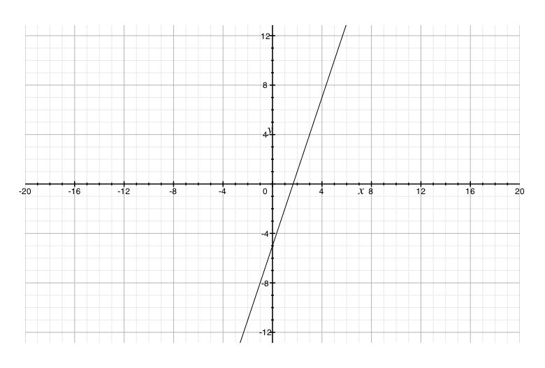
Graph y = 3x − 5
  • Identify slope
  • m = 3
  • Identify intercept
  • b = − 5
Graph utilizing slope and intercept
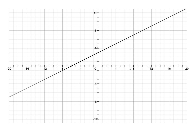
Graph y = [x/2] + 3
  • Identify slope
  • m = [1/2]
  • Identify intercept
  • b = 3
Graph utilizing slope and intercept

*These practice questions are only helpful when you work on them offline on a piece of paper and then use the solution steps function to check your answer.

Answer

Graphing Functions

Lecture Slides are screen-captured images of important points in the lecture. Students can download and print out these lecture slide images to do practice problems as well as take notes while watching the lecture.

  • Intro 0:00
  • Objectives 0:09
  • Graphing Functions 0:54
    • Using Slope-Intercept Form
    • Vertical Line Test
    • Determining the Domain
    • Determining the Range
  • Example 1 6:06
  • Example 2 7:18
  • Example 3 8:31
  • Example 4 11:04

Transcription: Graphing Functions

Welcome to www.educator.com.0000

In this lesson, we are going to work more with graphing functions now that we know a little bit more about them.0002

What you will see is that when it comes to graphing functions, we use a lot of the tools that we use with graphing just a normal equation.0012

We will see first how you can use a chart to plot a whole bunch of different points and graph out an entire function.0018

The good news is if you have a linear function, we can often use our tools for lines to shortcut that process.0027

Once we can look at the graph of the function, we will be able to determine whether it is truly a function using something like the vertical line test.0035

More importantly, once we have the graph of the function we can test out what its domain and range is just from looking at its graph.0044

Let us go ahead and take a look.0052

Graphing a function is the same process as graphing an equation.0058

We want to look at the relationship between the variables.0063

In order to do that, we can simply develop a table of values.0066

Remember doing this in our graphing of linear equation section, we may pick a lot of different values for x and see what the corresponding y value is.0071

The only difference that we might make with function is simply use different notation.0081

I would still pick a lot of different values for x but then I would simply see what the corresponding output is for my y values.0086

Always keep in mind that when we are dealing with our inputs, those are going to be our x values.0096

When we are dealing with our outputs, those are going to be our y values.0102

We will still be able to plot them on a coordinate axis.0107

Our x and y will correspond to the inputs and outputs of that function.0109

Now if a function represents a line then I have some good news for you.0119

You can use a lot of your techniques, especially about slope intercept form.0122

Here is a function written in slope intercept form, you can see that it still has the n being slope and it still has b being the y intercept.0127

The only change that I have done here is instead of writing out the y, I'm using my function notation.0141

This just gives us the name of the function and tells us that our independent variable here is x.0153

Since it is in slope intercept form, I could simply graph something like this by first using the y intercept as a starting point0161

and then using the slope to identify another point on that graph.0167

I have 2 points that I could connect them and then I'm good to go.0171

To determine if the graph is a function or not we can use what is known as the vertical line test.0182

The way the vertical line test works is you imagine a vertical line on the graph.0189

As long as it only crosses the graph in one spot, then you can consider it a function.0195

If the vertical line crosses the graph in only one spot and then we can consider it a function.0201

If it crosses in more than one spot that is where we will get into trouble.0208

Here I have two little diagrams, this one crosses here and here, we would say that this is not a function.0212

This one, it only crosses in one spot and if I was to move that dotted line into a different spot over here, it still crosses only one spot.0226

In that situation, I would say that this is a function.0247

To determine the domain and range of a function when you are looking at its graph,0262

think of tracing back all of the values that we used back to the x values on the x axis and back to the y values on the y axis.0266

This looks a little difficult to do at first but it is not that bad.0276

I imagine picking out some point out on the graph but if I am looking for the domain, I will trace it back to figure out what value on the x axis it came from.0281

If I pick another point, trace that back where did it come from on the x axis.0293

I do this for many, many different points I’m always tracing it back0299

What I'm looking to do is trace back essentially every single point on that graph.0303

Now what this would end up doing is I will end up plugging back many different points0310

and they would end up shading in the domain of all the x values that we have used in the function.0315

This one, if I trace this back trace it back, you can see that it creates that entire line.0327

In this part of the line out here comes from tracing back values on this side.0332

Even the ones that it can not see it, sure enough they traced all the way back.0338

In a similar fashion, you can figure out the range by taking these points and going to the y axis.0343

It is because the y’s represents the outputs, shading the axis, so you knew what was in your range.0349

That way we get a little bit better sense of how to graph functions and things about them.0365

Let us practice.0371

Let us use the vertical line test to see whether these following relations are functions or not.0373

The way a vertical line test works is we imagine a vertical line or test it to see if it crosses in only one spot.0379

On this first one over here, let us go ahead and put down a vertical line.0387

No matter where we move that vertical line, it looks like it will only end up crossing in one spot.0394

Since it only crosses once, we will say that it is a function.0402

With this one over here, when I put down a vertical line it is easy to see that it crosses in 2 spots.0412

It crosses in two spots, not a function.0422

The vertical line test says it must only cross in one spot at the most.0430

Let us go ahead and see if we can graph one of our linear functions.0440

In this one, it is a special type since it is linear.0443

We want to look at the form to see if that will help us out.0448

This one is written in slope intercept, I know that the y intercept is the 3 and I have a slope of -1/4.0451

Let us start with our first being right at 3 and from that point I will go down 1 to the right, 1, 2, 3, 4.0464

I have a second point, so I will connect the two.0473

There is my line.0483

I can also graph out this line by simply choosing a whole bunch of different values for x and evaluating them one at a time.0485

I simply use the slope intercept form because it will be a lot quicker.0495

I do want to point out that either way would be fine, just pick out some different things for x, plug them in and see what you will get for y.0500

You use the graph to determine the domain and range of the function.0513

This is unusual in that with last time we actually looked at the equation and tried to pick out what the natural domain was.0518

In here, I just have the graph and I have no idea what is being used in here but I can see the inputs and outputs.0525

Remember that is every single point on this graph here.0531

To first figure out the domain, I will imagine all the points and trace them back to this x axis.0536

What I'm doing is I’m figuring out what points we get shaded in on that x axis when I start tracing them all back.0545

What it looks like it is doing is it is tracing out a lot of different values here.0555

In fact, even my little point way out here we get trace back.0561

I will end up shading quite a bit of the x axis.0567

One thing to note is nothing is over on the side.0571

The reason why I have nothing over there, is there is no graph to trace back to the x axis.0576

Our domain looks like it would start here at -3 and it will go on and on forever from there.0581

We can use the same process to figure out what the range is.0596

We will simply take all our points now and trace them back to the y axis.0600

We will see what this shades in as we do this, bring that one back and you can see I’m shading a whole bunch of different values here.0605

In some places you might have more than one spot it traces back, but that is okay.0614

Let us see, keep shading going to the y axis, this guy will go back to -2.0620

Notice how below that I'm not going to shade anything on that part because there is no graph to trace back to the y-axis.0630

What do we have for our range? Well, the lowest value I have here is that -2.0642

We will start there and then it keeps going on from there since the rest of it is shaded.0648

Let us do one more domain and range.0660

Graph the relation and determine if it is a function then state its domain and range.0665

We got a little bit to do with this one, let us first just develop a graph in it.0670

This one is not a linear equation so I do not have too many shortcuts at my disposal.0675

I’m just going to end up creating a table of values to help me out.0680

Let us choose some different values like 4, 5, 8, and 13.0687

These values will make it a little bit easier to evaluate this.0698

If I was to use 4, I would end up with 2 × √4 - 4 or 2 × √0 which is 0.0702

That is one point I know is on my graph, at 4, 0.0721

Let us go ahead and put in our next value and that would be 5.0731

2 × √5-4 that would be 1, √1 = 1 so I have 2 as this value.0736

I will plug in 5 and I have 2 as my output.0748

Looking good, let us try some more.0752

Let us go ahead and put in the 8.0756

8 - 4 would be 4 and the √4 is 2, 2 × 2 =4.0762

This shows that when I put in 8 my output is 4.0773

Let us put in 1, 2, 3, 4, 5, 6, 7, 8, 4, there you go.0792

It looks like 13 is going to be off my-0803

13 - 4 would be 9, 2 × √9, 2 × 3 or 6.0815

That is another point on our graph.0823

Looking at our points, I might as well start putting them together so we can have a nice little curve right here.0827

Onto our first question, I was able to graph the relation, but is it a function or not?0835

Does it pass the vertical line test?0844

That is our question that we should be asking.0846

If we imagine a vertical line on here, does it cross once, more than once? What is happening?0849

What was this vertical line? I can see that no matter where I put it, it is only going to cross this graph in one spot.0856

I will say yes it is a function since it passes the vertical line test.0862

Now we have to figure out what is its domain and range.0877

What are all the inputs we could use and what are all the outputs?0880

In making this chart, I can already see some of the inputs that I used that you could potentially use even more than that.0884

If we trace back all these values, it also includes all the numbers between the ones we used.0890

I’m tracing things back to the x axis and it looks like I would shade in all of this.0896

This starts at 4 and continues on from there.0903

The domain would start at 4 and just go on from there, 4 to infinity.0907

If I take all of the same values then I start to trace them back to the y axis it will shade in a lot of other values but it looks like nothing less than 0.0917

We would shade in all that and now we have our range from 0 up to infinity.0933

You can see that graphing functions are the same process as just graphing any type of relation.0944

Keep track of your inputs and outputs.0949

If it is a special type of function like a linear function, then use your tools for graphing lines.0953

When it comes to the domain and range, look at your inputs and outputs by tracing all of the values back0959

and then show the intervals of all the numbers that should be included.0967

Thanks for watching www.educator.com.0970

Educator®

Please sign in to participate in this lecture discussion.

Resetting Your Password?
OR

Start Learning Now

Our free lessons will get you started (Adobe Flash® required).
Get immediate access to our entire library.

Membership Overview

  • Available 24/7. Unlimited Access to Our Entire Library.
  • Search and jump to exactly what you want to learn.
  • *Ask questions and get answers from the community and our teachers!
  • Practice questions with step-by-step solutions.
  • Download lecture slides for taking notes.
  • Track your course viewing progress.
  • Accessible anytime, anywhere with our Android and iOS apps.