INSTRUCTORS Carleen Eaton Grant Fraser Eric Smith

Eric Smith

Eric Smith

Variation & Proportion

Slide Duration:

Table of Contents

Section 1: Properties of Real Numbers
Basic Types of Numbers

30m 41s

Intro
0:00
Objectives
0:07
Basic Types of Numbers
0:36
Natural Numbers
1:02
Whole Numbers
1:29
Integers
2:04
Rational Numbers
2:38
Irrational Numbers
5:06
Imaginary Numbers
6:48
Basic Types of Numbers Cont.
8:09
The Big Picture
8:10
Real vs. Imaginary Numbers
8:30
Rational vs. Irrational Numbers
8:48
Basic Types of Numbers Cont.
10:55
Number Line
11:06
Absolute Value
11:44
Inequalities
12:39
Example 1
13:16
Example 2
17:30
Example 3
21:56
Example 4
24:27
Example 5
27:48
Operations on Numbers

19m 26s

Intro
0:00
Objectives
0:06
Operations on Numbers
0:25
Addition
0:53
Subtraction
1:33
Multiplication & Division
2:19
Exponents
3:24
Bases
4:04
Square Roots
4:59
Principle Square Roots
5:09
Perfect Squares
6:32
Simplifying and Combining Roots
6:52
Example 1
8:16
Example 2
12:30
Example 3
14:02
Example 4
16:27
Order of Operations

12m 6s

Intro
0:00
Objectives
0:06
The Order of Operations
0:25
Work Inside Parentheses
0:42
Simplify Exponents
0:52
Multiplication & Division from Left to Right
0:57
Addition & Subtraction from Left to Right
1:11
Remember PEMDAS
1:21
The Order of Operations Cont.
2:27
Example
2:43
Example 1
3:55
Example 2
5:36
Example 3
7:35
Example 4
8:56
Properties of Real Numbers

18m 52s

Intro
0:00
Objectives
0:07
The Properties of Real Numbers
0:23
Commutative Property of Addition and Multiplication
0:44
Associative Property of Addition and Multiplication
1:50
Distributive Property of Multiplication Over Addition
3:20
Division Property of Zero
4:46
Division Property of One
5:23
Multiplication Property of Zero
5:56
Multiplication Property of One
6:17
Addition Property of Zero
6:29
Why Are These Properties Important?
6:53
Example 1
9:16
Example 2
13:04
Example 3
14:30
Example 4
16:57
Section 2: Linear Equations
The Vocabulary of Linear Equations

12m 22s

Intro
0:00
Objectives
0:09
The Vocabulary of Linear Equations
0:44
Variables
0:52
Terms
1:09
Coefficients
1:40
Like Terms
2:18
Examples of Like Terms
2:37
Expressions
4:01
Equations
4:26
Linear Equations
5:04
Solutions
5:55
Example 1
6:16
Example 2
7:16
Example 3
8:45
Example 4
10:20
Solving Linear Equations in One Variable

28m 52s

Intro
0:00
Objectives
0:08
Solving Linear Equations in One Variable
0:34
Conditional Cases
0:51
Identity Cases
1:09
Contradiction Cases
1:30
Solving Linear Equations in One Variable Cont.
2:00
Addition Property of Equality
2:10
Multiplication Property of Equality
2:43
Steps to Solve Linear Equations
3:14
Example 1
4:22
Example 2
8:21
Example 3
12:32
Example 4
14:19
Example 5
17:25
Example 6
22:17
Solving Formulas

12m 2s

Intro
0:00
Objectives
0:06
Solving Formulas
0:18
Formulas
0:26
Use the Same Properties as Solving Linear Equations
1:36
Addition Property of Equality
1:55
Multiplication Property of Equality
1:58
Steps to Solve Formulas
2:43
Example 1
3:56
Example 2
6:09
Example 3
8:39
Applications of Linear Equations

28m 41s

Intro
0:00
Objectives
0:10
Applications of Linear Equations
0:43
The Six-Step Method to Solving Word Problems
0:55
Common Terms
3:12
Example 1
5:03
Example 2
9:40
Example 3
13:48
Example 4
17:58
Example 5
23:28
Applications of Linear Equations, Motion & Mixtures

24m 26s

Intro
0:00
Objectives
0:21
Motion and Mixtures
0:46
Motion Problems: Distance, Rate, and Time
1:06
Mixture Problems: Amount, Percent, and Total
1:27
The Table Method
1:58
The Beaker Method
3:38
Example 1
5:05
Example 2
9:44
Example 3
14:20
Example 4
19:13
Section 3: Graphing
Rectangular Coordinate System

22m 55s

Intro
0:00
Objectives
0:11
The Rectangular Coordinate System
0:39
The Cartesian Coordinate System
0:40
X-Axis
0:54
Y-Axis
1:04
Origin
1:11
Quadrants
1:26
Ordered Pairs
2:10
Example 1
2:55
The Rectangular Coordinate System Cont.
6:09
X-Intercept
6:45
Y-Intercept
6:55
Relation of X-Values and Y-Values
7:30
Example 2
11:03
Example 3
12:13
Example 4
14:10
Example 5
18:38
Slope & Graphing

27m 58s

Intro
0:00
Objectives
0:11
Slope and Graphing
0:48
Standard Form
1:14
Example 1
2:24
Slope and Graphing Cont.
4:58
Slope, m
5:07
Slope is Rise over Run
6:11
Don't Mix Up the Coordinates
8:20
Example 2
9:39
Slope and Graphing Cont.
14:26
Slope-Intercept Form
14:34
Example 3
16:55
Example 4
18:00
Slope and Graphing Cont.
19:00
Rewriting an Equation in Slope-Intercept Form
19:39
Rewriting an Equation in Standard Form
20:09
Slopes of Vertical & Horizontal Lines
20:56
Example 5
22:49
Example 6
24:09
Example 7
25:59
Example 8
26:57
Linear Equations in Two Variables

20m 36s

Intro
0:00
Objectives
0:13
Linear Equations in Two Variables
0:36
Point-Slope Form
1:07
Substitute in the Point and the Slope
2:21
Parallel Lines: Two Lines with the Same Slope
4:05
Perpendicular Lines: Slopes are Negative Reciprocals of Each Other
4:39
Perpendicular Lines: Product of Slopes is -1
5:24
Example 1
6:02
Example 2
7:50
Example 3
10:49
Example 4
13:26
Example 5
15:30
Example 6
17:43
Section 4: Functions
Introduction to Functions

21m 24s

Intro
0:00
Objectives
0:07
Introduction to Functions
0:58
Relations
1:03
Functions
1:37
Independent Variables
2:00
Dependent Variables
2:11
Function Notation
2:21
Function
3:43
Input and Output
3:53
Introduction to Functions Cont.
4:45
Domain
4:46
Range
4:55
Functions Represented by a Diagram
6:41
Natural Domain
9:11
Evaluating Functions
12:02
Example 1
13:13
Example 2
15:03
Example 3
16:18
Example 4
19:54
Graphing Functions

16m 12s

Intro
0:00
Objectives
0:09
Graphing Functions
0:54
Using Slope-Intercept Form
1:56
Vertical Line Test
2:58
Determining the Domain
4:20
Determining the Range
5:43
Example 1
6:06
Example 2
7:18
Example 3
8:31
Example 4
11:04
Section 5: Systems of Linear Equations
Systems of Linear Equations

25m 54s

Intro
0:00
Objectives
0:13
Systems of Linear Equations
0:46
System of Equations
0:51
System of Linear Equations
1:15
Solutions
1:35
Points as Solutions
1:53
Finding Solutions Graphically
5:13
Example 1
6:37
Example 2
12:07
Systems of Linear Equations Cont.
17:01
One Solution, No Solution, or Infinite Solutions
17:10
Example 3
18:31
Example 4
22:37
Solving a System Using Substitution

20m 1s

Intro
0:00
Objectives
0:09
Solving a System Using Substitution
0:32
Substitution Method
1:24
Substitution Example
2:35
One Solution, No Solution, or Infinite Solutions
7:50
Example 1
9:45
Example 2
12:48
Example 3
15:01
Example 4
17:30
Solving a System Using Elimination

19m 40s

Intro
0:00
Objectives
0:09
Solving a System Using Elimination
0:27
Elimination Method
0:42
Elimination Example
2:01
One Solution, No Solution, or Infinite Solutions
7:05
Example 1
8:53
Example 2
11:46
Example 3
15:37
Example 4
17:45
Applications of Systems of Equations

24m 34s

Intro
0:00
Objectives
0:12
Applications of Systems of Equations
0:30
Word Problems
1:31
Example 1
2:17
Example 2
7:55
Example 3
13:07
Example 4
17:15
Section 6: Inequalities
Solving Linear Inequalities in One Variable

17m 13s

Intro
0:00
Objectives
0:08
Solving Linear Inequalities in One Variable
0:37
Inequality Expressions
0:46
Linear Inequality Solution Notations
3:40
Inequalities
3:51
Interval Notation
4:04
Number Lines
4:43
Set Builder Notation
5:24
Use Same Techniques as Solving Equations
6:59
'Flip' the Sign when Multiplying or Dividing by a Negative Number
7:12
'Flip' Example
7:50
Example 1
8:54
Example 2
11:40
Example 3
14:01
Compound Inequalities

16m 13s

Intro
0:00
Objectives
0:07
Compound Inequalities
0:37
'And' vs. 'Or'
0:44
'And'
3:24
'Or'
3:35
'And' Symbol, or Intersection
3:51
'Or' Symbol, or Union
4:13
Inequalities
4:41
Example 1
6:22
Example 2
9:30
Example 3
11:27
Example 4
13:49
Solving Equations with Absolute Values

14m 12s

Intro
0:00
Objectives
0:08
Solve Equations with Absolute Values
0:18
Solve Equations with Absolute Values Cont.
1:11
Steps to Solving Equations with Absolute Values
2:21
Example 1
3:23
Example 2
6:34
Example 3
10:12
Inequalities with Absolute Values

17m 7s

Intro
0:00
Objectives
0:07
Inequalities with Absolute Values
0:23
Recall…
2:08
Example 1
3:39
Example 2
6:06
Example 3
8:14
Example 4
10:29
Example 5
13:29
Graphing Inequalities in Two Variables

15m 33s

Intro
0:00
Objectives
0:07
Graphing Inequalities in Two Variables
0:32
Split Graph into Two Regions
1:53
Graphing Inequalities
5:44
Test Points
6:20
Example 1
7:11
Example 2
10:17
Example 3
13:06
Systems of Inequalities

21m 13s

Intro
0:00
Objectives
0:08
Systems of Inequalities
0:24
Test Points
1:10
Steps to Solve Systems of Inequalities
1:25
Example 1
2:23
Example 2
7:28
Example 3
12:51
Section 7: Polynomials
Integer Exponents

44m 51s

Intro
0:00
Objectives
0:09
Integer Exponents
0:42
Exponents 'Package' Multiplication
1:25
Example 1
2:00
Example 2
3:13
Integer Exponents Cont.
4:50
Product Rule for Exponents
4:51
Example 3
7:16
Example 4
10:15
Integer Exponents Cont.
13:13
Power Rule for Exponents
13:14
Power Rule with Multiplication and Division
15:33
Example 5
16:18
Integer Exponents Cont.
20:04
Example 6
20:41
Integer Exponents Cont.
25:52
Zero Exponent Rule
25:53
Quotient Rule
28:24
Negative Exponents
30:14
Negative Exponent Rule
32:27
Example 7
34:05
Example 8
36:15
Example 9
39:33
Example 10
43:16
Adding & Subtracting Polynomials

18m 33s

Intro
0:00
Objectives
0:07
Adding and Subtracting Polynomials
0:25
Terms
0:33
Coefficients
0:51
Leading Coefficients
1:13
Like Terms
1:29
Polynomials
2:21
Monomials, Binomials, Trinomials, and Polynomials
5:41
Degrees
7:00
Evaluating Polynomials
8:12
Adding and Subtracting Polynomials Cont.
9:25
Example 1
11:48
Example 2
13:00
Example 3
14:41
Example 4
16:15
Multiplying Polynomials

25m 7s

Intro
0:00
Objectives
0:06
Multiplying Polynomials
0:41
Distributive Property
1:00
Example 1
2:49
Multiplying Polynomials Cont.
8:22
Organize Terms with a Table
8:23
Example 2
13:40
Multiplying Polynomials Cont.
16:33
Multiplying Binomials with FOIL
16:48
Example 3
18:49
Example 4
20:04
Example 5
21:42
Dividing Polynomials

44m 56s

Intro
0:00
Objectives
0:07
Dividing Polynomials
0:29
Dividing Polynomials by Monomials
2:10
Dividing Polynomials by Polynomials
2:59
Dividing Numbers
4:09
Dividing Polynomials Example
8:39
Example 1
12:35
Example 2
14:40
Example 3
16:45
Example 4
21:13
Example 5
24:33
Example 6
29:02
Dividing Polynomials with Synthetic Division Method
33:36
Example 7
38:43
Example 8
42:24
Section 8: Factoring Polynomials
Greatest Common Factor & Factor by Grouping

28m 27s

Intro
0:00
Objectives
0:09
Greatest Common Factor
0:31
Factoring
0:40
Greatest Common Factor (GCF)
1:48
GCF for Polynomials
3:28
Factoring Polynomials
6:45
Prime
8:21
Example 1
9:14
Factor by Grouping
14:30
Steps to Factor by Grouping
17:03
Example 2
17:43
Example 3
19:20
Example 4
20:41
Example 5
22:29
Example 6
26:11
Factoring Trinomials

21m 44s

Intro
0:00
Objectives
0:06
Factoring Trinomials
0:25
Recall FOIL
0:26
Factor a Trinomial by Reversing FOIL
1:52
Tips when Using Reverse FOIL
5:31
Example 1
7:04
Example 2
9:09
Example 3
11:15
Example 4
13:41
Factoring Trinomials Cont.
15:50
Example 5
18:42
Factoring Trinomials Using the AC Method

30m 9s

Intro
0:00
Objectives
0:08
Factoring Trinomials Using the AC Method
0:27
Factoring when Leading Term has Coefficient Other Than 1
1:07
Reversing FOIL
1:18
Example 1
1:46
Example 2
4:28
Factoring Trinomials Using the AC Method Cont.
7:45
The AC Method
8:03
Steps to Using the AC Method
8:19
Tips on Using the AC Method
9:29
Example 3
10:45
Example 4
16:50
Example 5
21:08
Example 6
24:58
Special Factoring Techniques

30m 14s

Intro
0:00
Objectives
0:07
Special Factoring Techniques
0:26
Difference of Squares
1:46
Perfect Square Trinomials
2:38
No Sum of Squares
3:32
Special Factoring Techniques Cont.
4:03
Difference of Squares Example
4:04
Perfect Square Trinomials Example
5:29
Example 1
7:31
Example 2
9:59
Example 3
11:47
Example 4
15:09
Special Factoring Techniques Cont.
19:07
Sum of Cubes and Difference of Cubes
19:08
Example 5
23:13
Example 6
26:12
Section 9: Quadratic Equations
Solving Quadratic Equations by Factoring

23m 38s

Intro
0:00
Objectives
0:08
Solving Quadratic Equations by Factoring
0:19
Quadratic Equations
0:20
Zero Factor Property
1:39
Zero Factor Property Example
2:34
Example 1
4:00
Solving Quadratic Equations by Factoring Cont.
5:54
Example 2
7:28
Example 3
11:09
Example 4
14:22
Solving Quadratic Equations by Factoring Cont.
18:17
Higher Degree Polynomial Equations
18:18
Example 5
20:22
Solving Quadratic Equations

29m 27s

Intro
0:00
Objectives
0:12
Solving Quadratic Equations
0:29
Linear Factors
0:38
Not All Quadratics Factor Easily
1:22
Principle of Square Roots
3:36
Completing the Square
4:50
Steps for Using Completing the Square
5:15
Completing the Square Works on All Quadratic Equations
6:41
The Quadratic Formula
7:28
Discriminants
8:25
Solving Quadratic Equations - Summary
10:11
Example 1
11:54
Example 2
13:03
Example 3
16:30
Example 4
21:29
Example 5
25:07
Equations in Quadratic Form

16m 47s

Intro
0:00
Objectives
0:08
Equations in Quadratic Form
0:24
Using a Substitution
0:53
U-Substitution
1:26
Example 1
2:07
Example 2
5:36
Example 3
8:31
Example 4
11:14
Quadratic Formulas & Applications

29m 4s

Intro
0:00
Objectives
0:09
Quadratic Formulas and Applications
0:35
Squared Variable
0:40
Principle of Square Roots
0:51
Example 1
1:09
Example 2
2:04
Quadratic Formulas and Applications Cont.
3:34
Example 3
4:42
Example 4
13:33
Example 5
20:50
Graphs of Quadratics

26m 53s

Intro
0:00
Objectives
0:06
Graphs of Quadratics
0:39
Axis of Symmetry
1:46
Vertex
2:12
Transformations
2:57
Graphing in Quadratic Standard Form
3:23
Example 1
5:06
Example 2
6:02
Example 3
9:07
Graphs of Quadratics Cont.
11:26
Completing the Square
12:02
Vertex Shortcut
12:16
Example 4
13:49
Example 5
17:25
Example 6
20:07
Example 7
23:43
Polynomial Inequalities

21m 42s

Intro
0:00
Objectives
0:07
Polynomial Inequalities
0:30
Solving Polynomial Inequalities
1:20
Example 1
2:45
Polynomial Inequalities Cont.
5:12
Larger Polynomials
5:13
Positive or Negative Intervals
7:16
Example 2
9:01
Example 3
13:53
Section 10: Rational Equations
Multiply & Divide Rational Expressions

26m 41s

Intro
0:00
Objectives
0:09
Multiply and Divide Rational Expressions
0:44
Rational Numbers
0:55
Dividing by Zero
1:45
Canceling Extra Factors
2:43
Negative Signs in Fractions
4:52
Multiplying Fractions
6:26
Dividing Fractions
7:17
Example 1
8:04
Example 2
14:01
Example 3
16:23
Example 4
18:56
Example 5
22:43
Adding & Subtracting Rational Expressions

20m 24s

Intro
0:00
Objectives
0:07
Adding and Subtracting Rational Expressions
0:41
Common Denominators
0:52
Common Denominator Examples
1:14
Steps to Adding and Subtracting Rational Expressions
2:39
Example 1
3:34
Example 2
5:27
Adding and Subtracting Rational Expressions Cont.
6:57
Least Common Denominators
6:58
Transitioning from Fractions to Rational Expressions
9:08
Identifying Least Common Denominators for Rational Expressions
9:56
Subtracting vs. Adding
10:41
Example 3
11:19
Example 4
12:36
Example 5
15:08
Example 6
16:46
Complex Fractions

18m 23s

Intro
0:00
Objectives
0:09
Complex Fractions
0:37
Dividing to Simplify Complex Fractions
1:10
Example 1
2:03
Example 2
3:58
Complex Fractions Cont.
9:15
Using the Least Common Denominator to Simplify Complex Fractions
9:16
Both Methods Lead to the Same Answer
10:07
Example 3
10:42
Example 4
14:28
Solving Rational Equations

16m 24s

Intro
0:00
Objectives
0:07
Solving Rational Equations
0:23
Isolate the Specified Variable
1:23
Example 1
1:58
Example 2
5:00
Example 3
8:23
Example 4
13:25
Rational Inequalities

18m 54s

Intro
0:00
Objectives
0:06
Rational Inequalities
0:18
Testing Intervals for Rational Inequalities
0:38
Steps to Solving Rational Inequalities
1:05
Tips to Solving Rational Inequalities
2:27
Example 1
3:33
Example 2
12:21
Applications of Rational Expressions

20m 20s

Intro
0:00
Objectives
0:07
Applications of Rational Expressions
0:27
Work Problems
1:05
Example 1
2:58
Example 2
6:45
Example 3
13:17
Example 4
16:37
Variation & Proportion

27m 4s

Intro
0:00
Objectives
0:10
Variation and Proportion
0:34
Variation
0:35
Inverse Variation
1:01
Direct Variation
1:10
Setting Up Proportions
1:31
Example 1
2:27
Example 2
5:36
Variation and Proportion Cont.
8:29
Inverse Variation
8:30
Example 3
9:20
Variation and Proportion Cont.
12:41
Constant of Proportionality
12:42
Example 4
13:59
Variation and Proportion Cont.
16:17
Varies Directly as the nth Power
16:30
Varies Inversely as the nth Power
16:53
Varies Jointly
17:09
Combining Variation Models
17:36
Example 5
19:09
Example 6
22:10
Section 11: Radical Equations
Rational Exponents

14m 32s

Intro
0:00
Objectives
0:07
Rational Exponents
0:32
Power on Top, Root on Bottom
1:05
Example 1
1:37
Rational Exponents Cont.
4:04
Using Rules from Exponents for Radicals as Exponents
4:05
Combining Terms Under a Single Root
4:50
Example 2
5:21
Example 3
7:39
Example 4
11:23
Example 5
13:14
Simplify Rational Exponents

15m 12s

Intro
0:00
Objectives
0:07
Simplify Rational Exponents
0:25
Product Rule for Radicals
0:26
Product Rule to Simplify Square Roots
1:11
Quotient Rule for Radicals
1:42
Applications of Product and Quotient Rules
2:17
Higher Roots
2:48
Example 1
3:39
Example 2
6:35
Example 3
8:41
Example 4
11:09
Adding & Subtracting Radicals

17m 22s

Intro
0:00
Objectives
0:07
Adding and Subtracting Radicals
0:33
Like Terms
1:29
Bases and Exponents May be Different
2:02
Bases and Powers Must be Same when Adding and Subtracting
2:42
Add Radicals' Coefficients
3:55
Example 1
4:47
Example 2
6:00
Adding and Subtracting Radicals Cont.
7:10
Simplify the Bases to Look the Same
7:25
Example 3
8:23
Example 4
11:45
Example 5
15:10
Multiply & Divide Radicals

19m 24s

Intro
0:00
Objectives
0:08
Multiply and Divide Radicals
0:25
Rules for Working With Radicals
0:26
Using FOIL for Radicals
1:11
Don’t Distribute Powers
2:54
Dividing Radical Expressions
4:25
Rationalizing Denominators
6:40
Example 1
7:22
Example 2
8:32
Multiply and Divide Radicals Cont.
9:23
Rationalizing Denominators with Higher Roots
9:25
Example 3
10:51
Example 4
11:53
Multiply and Divide Radicals Cont.
13:13
Rationalizing Denominators with Conjugates
13:14
Example 5
15:52
Example 6
17:25
Solving Radical Equations

15m 5s

Intro
0:00
Objectives
0:07
Solving Radical Equations
0:17
Radical Equations
0:18
Isolate the Roots and Raise to Power
0:34
Example 1
1:13
Example 2
3:09
Solving Radical Equations Cont.
7:04
Solving Radical Equations with More than One Radical
7:05
Example 3
7:54
Example 4
13:07
Complex Numbers

29m 16s

Intro
0:00
Objectives
0:06
Complex Numbers
1:05
Imaginary Numbers
1:08
Complex Numbers
2:27
Real Parts
2:48
Imaginary Parts
2:51
Commutative, Associative, and Distributive Properties
3:35
Adding and Subtracting Complex Numbers
4:04
Multiplying Complex Numbers
6:16
Dividing Complex Numbers
8:59
Complex Conjugate
9:07
Simplifying Powers of i
14:34
Shortcut for Simplifying Powers of i
18:33
Example 1
21:14
Example 2
22:15
Example 3
23:38
Example 4
26:33
Loading...
This is a quick preview of the lesson. For full access, please Log In or Sign up.
For more information, please see full course syllabus of Algebra 1
Bookmark & Share Embed

Share this knowledge with your friends!

Copy & Paste this embed code into your website’s HTML

Please ensure that your website editor is in text mode when you paste the code.
(In Wordpress, the mode button is on the top right corner.)
  ×
  • - Allow users to view the embedded video in full-size.
Since this lesson is not free, only the preview will appear on your website.
  • Discussion

  • Answer Engine

  • Study Guides

  • Practice Questions

  • Download Lecture Slides

  • Table of Contents

  • Transcription

  • Related Books

Lecture Comments (4)

1 answer

Last reply by: Professor Eric Smith
Mon Aug 12, 2019 11:30 AM

Post by Sean Zhang on August 12, 2019

in the first example, you wrote is as x1,y1,x2,y1

1 answer

Last reply by: Professor Eric Smith
Mon Oct 19, 2015 11:45 AM

Post by Khanh Nguyen on October 17, 2015

In practice question #7, in the answer, it says quardrants.
In practice question #8, in the answer, it says quadrant instead of quadrants.
Could you please fix it?
:^D

Variation & Proportion

  • Variation is a connection between two variables such that one is a constant multiple of the other.
  • Some of the major types of variation are
    • Direct variation y = kx
    • Inverse variation y=k/x
    • Joint variation y=kxz
  • Variation can be modeled using proportions, or simple formulas. Make sure you label what the variables represent, and to line them up carefully.
  • Variation can also be used to connect variables when they are squared, or taken to a root. Watch for clues in the wording of the problem to help identify these.
  • Multiple types of variation can be combined into a single problem. For these make sure variables connected directly, or jointly end up in the numerator. Variables connected inversely should be put in the denominator.

Variation & Proportion

Assume that y varies inversely with x. If x1 = 15 when y1 = 10 find x2 when y2 = − 6
  • x1y1 = x2y2
  • ( 15 )( 10 ) = x2( − 6 )
  • [150/( − 6)] = x2
x2 = − 25
Assume that y varies inversely with x. If x1 = 7 when y1 = 13, find y2 when x2 = 11
  • x1y1 = x2y2
  • ( 7 )( 13 ) = 11y2
[91/11] = y2
Assume that y varies inversely with x. If x1 = 14 when y1 = 7 find x2 when y2 = − [1/4]
  • ( 14 )( 7 ) = x2( − [1/4] )
x2 = − 392
Assume that y varies inversely with x. If x1 = 8 when y1 = 4 find y2 when x2 = − [4/6]
  • ( 8 )( 4 ) = x2( − [4/6] )
  • ( − [6/4] )( 8 )( 4 ) = x2
x2 = − 48
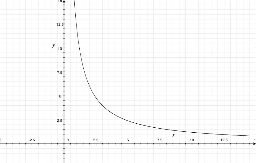
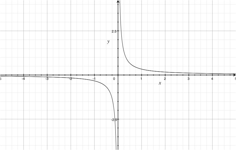
Graph the inverse variation xy = 12. Assume x to be only positive
  • Identify equivalent form to xy = ky = [12/x]
  • Make a table of points
    x
    line
    1
    2
    3
    4
    5
    y
    line
    12
    6
    4
    3
    [12/5]
Graph utilizing points
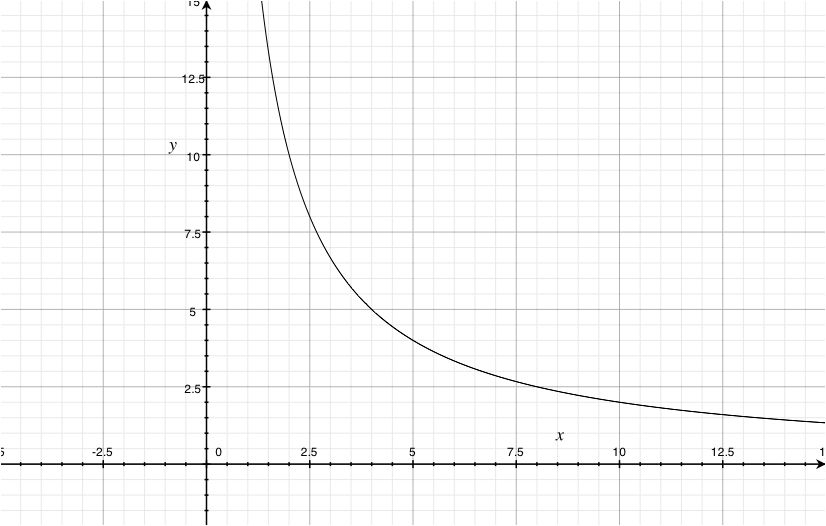
Graph the inverse variation 2xy = 40. Assume x to be only positive
  • Identify equivalent form to xy = ky = [20/x]
  • Make a table of points
    x
    line
    1
    2
    3
    4
    5
    y
    line
    20
    10
    [20/3]
    5
    4
Graph utilizing points
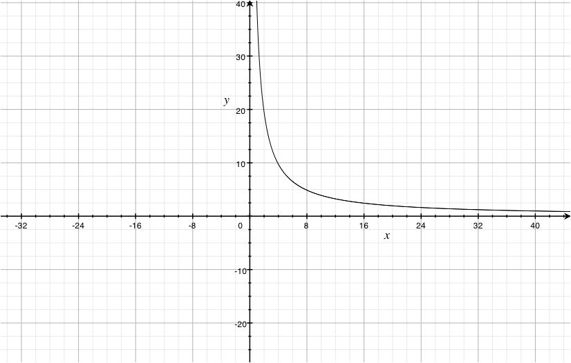
Graph the inverse variation x( − [y/3]) = − 13. Assume x to be only positive
  • Identify equivalent form to xy = ky = [39/x]
  • Make a table of points
    x
    line
    1
    4
    7
    10
    13
    y
    line
    39
    [39/4]
    [39/7]
    [39/10]
    3
Graph utilizing points
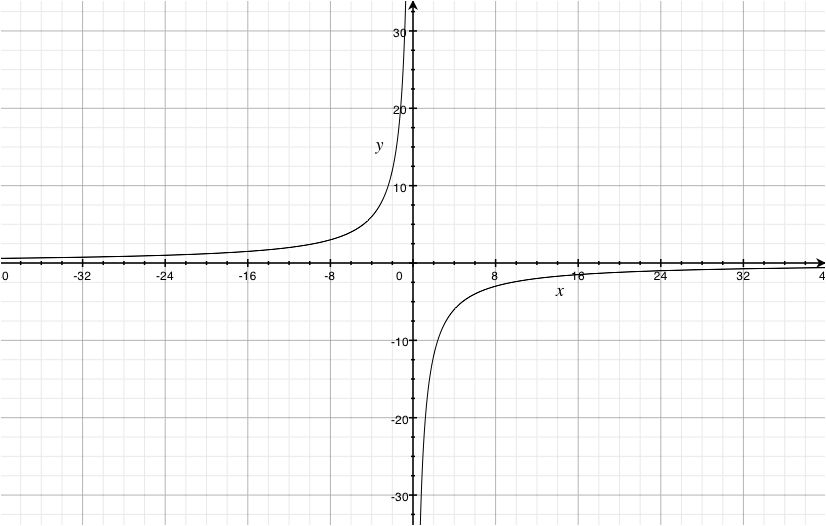
Identify the quadrants of the branches in the function xy = − 24
  • Identify equivalent form to xy = ky = [( − 24)/x]
  • Make a table of points
    x
    line
    − 12
    − 8
    − 4
    4
    8
    12
    y
    line
    2
    3
    6
    − 6
    − 3
    − 2
  • Graph utilizing points
Quardrants II and IV
Identify the quadrants of the branches in the function xy = [1/3]
  • Identify equivalent form to xy = ky = [1/3x]
  • Make a table of points
    x
    line
    − 3
    − 2
    − 1
    1
    2
    3
    y
    line
    − [1/9]
    − [1/6]
    − [1/3]
    [1/3]
    [1/6]
    [1/9]
  • Graph utilizing points
Quadrant I and III
Graph the inverse variation 8x([y/4]) = 56
  • Identify equivalent form to xy = ky = [28/x]
  • Make a table of points
    x
    line
    − 24
    − 16
    − 8
    8
    16
    24
    y
    line
    − [7/6]
    − [7/4]
    − [7/2]
    [7/2]
    [7/4]
    [7/6]
Graph utilizing points

*These practice questions are only helpful when you work on them offline on a piece of paper and then use the solution steps function to check your answer.

Answer

Variation & Proportion

Lecture Slides are screen-captured images of important points in the lecture. Students can download and print out these lecture slide images to do practice problems as well as take notes while watching the lecture.

  • Intro 0:00
  • Objectives 0:10
  • Variation and Proportion 0:34
    • Variation
    • Inverse Variation
    • Direct Variation
    • Setting Up Proportions
  • Example 1 2:27
  • Example 2 5:36
  • Variation and Proportion Cont. 8:29
    • Inverse Variation
  • Example 3 9:20
  • Variation and Proportion Cont. 12:41
    • Constant of Proportionality
  • Example 4 13:59
  • Variation and Proportion Cont. 16:17
    • Varies Directly as the nth Power
    • Varies Inversely as the nth Power
    • Varies Jointly
    • Combining Variation Models
  • Example 5 19:09
  • Example 6 22:10

Transcription: Variation & Proportion

Welcome back to www.educator.com.0000

In this lesson we are going to take a look at a very interesting application of our rational.0002

We will look at variation and proportion.0006

We will have to do a little bit of work just to explain what I mean by the word variation.0012

We will break this down into few other things.0017

We will look at direct variation, inverse variation, and combined variation.0019

This particular section is filled with lots of different word problems all of them involving variation.0025

Let us see what we can do.0032

When you hear that word variation we are talking about a connection between two variables,0036

such that one is a constant multiple of the other.0041

You will see some nice handy formulas that will highlight how one is a constant multiple of the other.0044

If you are looking for little bit more intuition on the situation then you can grasp on to that.0050

Intuitively a variation can be thought of as a special connection and the two basic types are direct and inverse.0055

In this connection when one quantity goes up then the other one would go down.0063

In that one I'm talking about an inverse variation.0069

If I’m thinking about those two quantities when one goes up and the other one goes up as well, that will be an example of a direct variation.0075

It is how one affects the other one and they could be moving in the same direction our going in the opposite directions.0084

To model this type of situation that has variation in it, you can end up setting up a proportion.0094

Be very careful on where you put each of the individual components and make sure you line them up correctly.0100

To model a direct variation, you could use the following proportion x1 / y1 = x2 / y2.0107

The way want to interpret those subscripts that you are seeing on everything is that all of the values with a subscript of 1 involved one situation.0116

Everything with the 2 involves a second situation.0126

Since the x are both on the top that will be from one particular type of thing and y will be from another type of things.0133

We will line those up to make sure that they at least agree.0142

It seems a little vague but let us get into an example0148

and you will see how I do set this up using a proportion and how everything does line up.0151

This one says that an objects weight on the moon varies directly as its weight on earth.0156

Neil Armstrong, the first person to step on the mood weighed 360 pounds on Earth, when he is on the moon he was only 60 pounds.0163

The question is if we take just an average person who weighs 186 pounds, what will their weight be if they go to the moon?0174

We have that this is a direct variation because it pointed out and says it is a direct variation.0186

Let us just think a little bit and see if that makes sense.0192

Intuitively in a direct variation when one quantity goes up then should be the other one.0196

When one quantity goes down, then so should the other one.0201

That is what is going on with our moon weight.0204

If I decide to go on and get heavier and heavier on Earth, that same thing is going to happen on the moon.0207

I will get heavier and heavier on the moon.0214

This is a type of direct proportion.0217

Let us see what we can set up.0223

x1 / y1 = x2 / y20224

To help out I’m going to highlight two things, we will go ahead and keep our Earth weights on top0231

and we will go ahead and put our moon weights on the bottom.0238

Let us look at our first situation with our Neil Armstrong.0245

He weighed 360 pounds on Earth, and only 60 pounds on the moon.0250

360 on Earth and 60 on the moon.0255

I will compare that with our average person there.0267

They weigh 186 pounds on the Earth, but we have no idea how much they weigh on the moon.0270

I'm going to put that as my unknown.0277

Everything on the tops of these fractions represents an earth weight and everything on the bottom represents a moon weight.0280

You can see that we have developed one of these rational equations and now we simply have to solve it.0287

This one is not too bad if you go ahead and reduce that fraction on the left, it goes in there 6 times.0292

We can multiply both sides by x.0301

I have 6x = 186.0308

Finally dividing both sides by 6 I will get that x =31.0316

This reveals how much that average person, the 186 pounds would weigh when they are on the moon.0327

There are lots of other types of situations that could involve a direct proportion and they might not come out and say its direct proportion.0338

Look for clues along the way to help out.0344

This one says that a maintenance bill for a shopping center containing 270,000 ft2 is $45,000.0348

What is the bill of the first store in the center that is only 4800 ft2?0356

Let us think of what type of a variation this should be.0361

If I have a large store as a part of the shopping mall and I will have to end up paying a much larger maintenance or bill because of my larger store.0366

If I have a small store then my bill should be very small.0378

Those quantities are moving in the same direction.0382

I’m going to say this is an example of direct variation.0385

We will set it up using our proportion.0392

We want to keep things straight.0403

What do each of these quantities represent?0405

Let us say the top will be our square footage and we will make the bottom the bill.0409

How much it cost?0421

Let us go ahead and substitute some of this information we have.0424

If I’m looking at the entire shopping center I know how big it is and I know the bill for the entire place.0427

270,000, 45,000 and now I can look at my much smaller store, it only has 4800 ft20435

and this one we have no idea what the bill is so I will leave that one as my unknown.0453

I think we can do a little bit of simplifying with this one as well.0459

I will divide these two and we get 6 and I need to just solve this rational equation which is not too bad as long as we multiply both sides by x.0464

I have 6x = 4800.0481

Divide both sides by 6 and then I think we will have our solution x =800.0488

Even if they do not come out and tell you what type of variation is going on here,0497

look at the values present to see if things are moving in the same direction, or in opposite directions.0502

For inverse variation we want to make sure that if one quantity goes up, the other one goes down.0510

One way that we can model it now with our proportions is to set up like this.0516

We will go ahead and use us a subscript for one situation and we will put them on opposite sides of our equal sign.0521

We will get that inverse relationship.0528

When one goes up, the other one will go down.0531

For our second situation we will put these on two opposite sides of the equal sign.0535

One thing that will not change is that both of these x will represent the same type of thing0541

and both of these y will still represent the same type of thing.0546

We can definitely note that the things are on opposite sides of the equal sign for these given situations.0550

For my inverse variation problem I will look at the current in a circuit and we are told that it varies inversely with the resistance.0562

If I have a current that is 30 amps when the resistance is 5 ohms, find the current for resistance of 25 ohms.0572

I have a lot of things in here and we just want to keep track of each of them.0581

Let us see if we can highlight each of these situations.0586

The current is 30 amps when the resistance is 5.0589

We will be looking for the current when the resistance is 25.0596

Let us get our proportion out here.0605

I’m using these little subscripts and put them on opposite sides.0611

Onto the first situation, we will keep everything on the top.0615

Let us say that is our resistance, we will put everything on the bottom as the current.0624

Our first situation, we know that the current is going to be 30 when the resistance is 5.0635

In that situation I will put my 5 and 30.0641

For the other situation I want to figure out what the current is.0647

I have no idea what that is but I know that the resistance is 25 ohms.0651

This is my initial proportion that I have set up.0657

All we have to do is go through the process of solving it.0661

This one is not too bad.0664

Let us multiply both sides by 30x and see what is left over.0666

30 × 5, since the x will cancel out equals 25 × x since the 30 cancel out.0673

Okay looking pretty good.0688

Also 5 × 30 =150 equals 25x and we can simply divide both sides by 25 to get our answer.0690

The current is 6 amps.0708

When dealing with these variation problems always look at your solution and see if it makes sense in the context of the problem.0722

One thing that I'm noticing in here is that I start off with a resistance of 5 and a current of 30.0729

One thing I'm doing with my current is that I'm lowering it, and I'm taking it from 30 down to 25.0736

Since I have an inverse relationship that is going to have an effect on our amps is the current.0744

That should bring it up.0751

Originally I started with 5 and I can see my answer is 6.0753

It did go up and things are working in the right direction.0757

Since earlier, we said that it variation is relationship when one is a constant multiple of the other.0764

We can model this using some nice formulas.0769

For direct variation you can use the formula y = k × x.0773

For your inverse variation, you could use y = k ÷ x.0779

We have two variables in each of these equations that we are looking at connecting are the x and y.0785

The k in each of these is known as our constant of proportionality.0791

It connects how they are related.0795

A lot of problems that you will end up doing with these variations, if you want to use these formulas0799

then you will end up going through three steps to figure out what is going on.0806

You might first go ahead and identify what type of variation you are using so that you can take one of these formulas.0811

Then you will end up using a little bit of known information to go ahead and solve for that constant of proportionality, k.0818

Once you know what k is, then you can usually figure out some new information by substituting it into the formula.0825

I got a couple of examples where we are going through these 3 steps.0832

Let us first just see an example of using an inverse of variation using one of these formulas.0840

This one says that the speed of water through a hose is inversely proportional to a cross section of the area of the hose.0846

If a person places their thumb on the end of the hose and decreases the area by 75%, what does this do the speed of the water?0855

Let us think about what we got here.0867

We are looking for a connection among the cross area section of the hose and the speed of the water.0868

We are told that they are set up inversely so when one goes down, the other one should go up.0876

For decreasing the area then we should expect it to increase the speed of the water.0879

In fact we can be a little bit more precise, but despite playing around with those formulas for a little bit.0887

Our relationship is that the speed of the water is inversely proportional to a cross section of the area.0893

Maybe x = k/a.0900

I'm going to decrease the area by 75%, one way that I could model that is by simply multiplying our area by what is left over, 25%.0905

Let us relate this to the original before I manipulated it.0923

25 is the same as ¼ I'm dividing by ¼.0928

When you divide by a fraction that is the same as multiplying.0936

This is multiply by 4.0943

Now we can see the difference between the original situation.0947

The area decreased by 75%.0956

They are almost exactly the same but in the second situation, it is 4 times as much.0966

It will actually increase the speed by 4 times.0971

There are lots of other types of variations that you can go ahead and work into a problem.0978

Some of these will look similar to previous types that we covered.0982

Let us go through how each of these are connected.0984

If I say that y varies directly to some power of x then there are some k that connects those two things.0990

You will notice that it looks like our direct proportion only since we are dealing with an nth power,0997

like a 3rd power 4th power that we put that exponent right on the other variable.1004

Our y varies inversely as the nth power looks much like our inverse relationship as well.1013

But since we are doing it to the nth power, notice how we put that exponent right on the other variable.1020

In this one is a new one that involves a few more variables, this is our joint variation.1029

y varies jointly as x and z so more than one variable now.1034

If there some sort of positive constant such that y = k × x × z.1039

In this one the k is our constant and the variables are being connected, the y, x, and z.1046

You can start mixing and matching these various different types of variation.1057

The reason why that we do not want to start mixing and matching them is we can get some more complicated models.1064

With these more complicated models we are hoping to be able to more accurately model what is happening in a real life situation.1071

Usually it does a better job than any one variation could do by itself.1079

The key when putting all of those different types of variations together is to look for clues in the actual problem itself.1085

Here is a formula that I have it is T = k × x × z3 /√y .1092

Here is how I could describe that problem using the language of these variations.1100

The k right here is my constant of proportionality and we are looking to get it connect together the t, x, z, and y.1107

Here is what I can say, the t varies jointly with x and z3.1116

It is telling me that I have my constant of proportionality but the x and z should end up in the top and the z should be cubed.1123

t also varies inversely with the √y.1133

Since it is an inverse relationship I will put that one in the bottom and make sure to put in that square root.1138

Watch for those keywords so we can figure out where we should put things.1145

Let us try some of these variation problems and watch as I walk through the three steps of1151

starting with some template solving for our constant of proportionality, k and the last part figure out some new information.1155

What do I know so far?1167

I know that y varies jointly as x and z.1168

Just on that little part, let us go ahead and make a nice formula.1173

y varies jointly as x and z.1177

y = 12 when x = 9 and z = 3.1184

I can use that information right there to go ahead and solve for my constant of proportionality.1191

y =12, x = 9, z= 31198

The only unknown I have in there is that k value.1206

We will combine things I will get 27 divide both sides by 27 and then maybe reduce that by dividing the top and bottom by 3.1210

Now that we know much more I can end up revising our formula.1228

y = xz and now I can say that the k value is this 4/9.1236

Now that we know about our constant of proportionality, let us find z when y = 6 and x = 15.1244

We will substitute those directly in there and you will see the only unknown I have left will be that z.1253

Y= 6, 4/9 × 15 and we are not sure what z is now we have to solve for it.1259

A little bit of work.1270

I think I can cancel out an extra 3 here.1272

I have 6 = 20/3 × z we could multiply both sides by 3.1276

I will get rid of those 3, 18 = 20z.1292

Lastly let us go and divide both sides by 20.1298

18 ÷ 20 =z1301

We will just go ahead and put that into lowest terms.1306

Divide the top and bottom by 2 and I know that 9/10 is equal to z.1310

If you follow along we start with some sort of template for our variation, we solved for our unknown constant of proportionality k.1316

We have used it to figure out some new information about the other variables.1325

For this last type of example let us look at one that is a little bit more of a word problem.1331

This one says that we have the maximum load of the beam and how much you can support varies jointly1336

with the width of the beam and the square of its depth, but it varies inversely as the length of the beam.1343

Some of that initial information there is just giving us a formula for how everything is connected.1352

We will definitely set up the equation that will model that situation.1358

Let us continue on.1364

Assume that a beam that is 3 feet wide, 2 feet deep, 30 feet long and it can support 84 pounds.1365

What is the maximum load a similar beam can support if it is 2 feet wide, 5 feet deep and 100 feet long?1371

A lot of information is floating around there.1378

Let us start off by seeing if we can set up this formula.1381

The maximum load that a beam can support varies jointly as the width of the beam and the square of its depth.1385

Since this is a jointly, we are talking about k × width × the square of its depth or d2.1395

It varies inversely with the length, I will put the length on the bottom.1408

This part here is our formula that we will end up using.1413

Assuming that a beam is 3 feet wide, 2 feet deep and 30 feet long, and it can support 84 pounds,1421

let us use that to figure out our unknown constant sitting right here that k.1426

I know it can support 84 pounds, we do not know k.1432

3 feet wide, I put that in for width, 2 feet deep and it is 30 long.1440

The only unknown is that k.1448

Let us go ahead and simplify it just little bit in here.1451

I have 3 × 22 and 22 is 4 = 121455

I can get that k a little bit more by itself if I multiply both sides by 30, 84 × 30.1463

Let us go ahead and put those together and see that would be 2520.1473

Divide both sides by 12.1483

That is where we have been able to figure out what that unknown constant is.1488

Now that I have that I can go back to the original formula.1494

M = 210w × d2 / l1498

We will use this new formula to figure out a little bit of known information.1506

We will look at it for the other beam where we are looking for its maximum load if we know its width, depth, and its length.1512

Let us give it a try.1520

That formula we developed was its maximum load = 210 × width × d2 / length.1525

Let us put in our information.1536

For this new beam, its width is 2 feet and its depth is 5.1541

It also has a length of 100.1549

As soon as we simplify all that we will be able to figure out what its maximum load should be.1551

210 × 2 = 420 × 25 ÷ 1001558

Let us do some simplifying here 420 × 25 = 10500 ÷ 100 and looks like this reduces to 105.1573

This new beam can support a maximum of 105 pounds.1593

Being able to recognize various different types of variation1599

and combine them all together is essential for some more complicated problems.1602

Remember that if you have those nice formulas then you can go through 3 steps.1607

One, build a formula or equation that models the situation, solve for your unknown k1611

and finally use some new information to figure out some more information about the problem.1617

Thank you for watching www.educator.com.1622

Educator®

Please sign in to participate in this lecture discussion.

Resetting Your Password?
OR

Start Learning Now

Our free lessons will get you started (Adobe Flash® required).
Get immediate access to our entire library.

Membership Overview

  • Available 24/7. Unlimited Access to Our Entire Library.
  • Search and jump to exactly what you want to learn.
  • *Ask questions and get answers from the community and our teachers!
  • Practice questions with step-by-step solutions.
  • Download lecture slides for taking notes.
  • Track your course viewing progress.
  • Accessible anytime, anywhere with our Android and iOS apps.