Raffi Hovasapian

Double Integrals

Slide Duration:

Table of Contents

Section 1: Vectors

Points & Vectors

28m 23s

Intro

0:00

Points and Vectors

1:02

A Point in a Plane

1:03

A Point in Space

3:14

Notation for a Space of a Given Space

6:34

Introduction to Vectors

9:51

Adding Vectors

14:51

Example 1

16:52

Properties of Vector Addition

18:24

Example 2

21:01

Two More Properties of Vector Addition

24:16

Multiplication of a Vector by a Constant

25:27

Scalar Product & Norm

30m 25s

Intro

0:00

Scalar Product and Norm

1:05

Introduction to Scalar Product

1:06

Example 1

3:21

Properties of Scalar Product

6:14

Definition: Orthogonal

11:41

Example 2: Orthogonal

14:19

Definition: Norm of a Vector

15:30

Example 3

19:37

Distance Between Two Vectors

22:05

Example 4

27:19

Multivariable Calculus Double Integrals

Name: Multivariable Calculus: Double Integrals
Brand: Educator.com
Price: 35 USD
Availability: InStock

Section 7: Double Integrals: Lecture 1 | 29:46 min

Lecture Description

Next Lecture

Previous Lecture

Discussion
Answer Engine
Practice Questions
Download Lecture Slides
Table of Contents
Transcription
Related Books

Lecture Comments (9)

	1 answer Last reply by: Professor Hovasapian Fri Aug 22, 2014 8:27 PM Post by Denny Yang â™• [Moderator] on August 19, 2014 Also in example 3, you made a minor calculation error. You wrote: The integral of(2x^3 - 12x^2 +19x, x, (3/2), 3 ). It should have been (2x^3 - 12x^2 +18x, x, (3/2), 3 ). The [ x, (3/2), 3 ] is the variable we are integrating and the lower bound and upper bound. Typing it just like you would on a Ti-89 Calculator.
	1 answer Last reply by: Professor Hovasapian Fri Aug 22, 2014 8:23 PM Post by Denny Yang â™• [Moderator] on August 19, 2014 Q. ii) Integrate âˆ« âˆ’ Ï€\protect\mathord/ \protect phantom Ï€2 / 20 ey dx. What is this?
	1 answer Last reply by: Professor Hovasapian Mon May 13, 2013 12:53 AM Post by Josh Winfield on May 12, 2013 Hello Raffi, Can you just clarify why in example 3 you put the limit of integration for dx as (3-y) on the bottom and (y) on the top. I had them the other way around but im wrong but i cant figure out why?
	0 answers Post by Justin Dehorty on February 23, 2013 How do I find the Lower and Upper Sums? Apparently this is another way to calculate double integrals, but I don't understand how to set up the sigmas properly.
	1 answer Last reply by: Professor Hovasapian Sat Dec 29, 2012 5:01 PM Post by Alexander Rekitsanov Alexander Rekitsanov on December 15, 2012 I think that the region the prof is integrating is wrong in example 3. in the question it is stating that region that is bounded by y=0 ,y=x and y=-x+3 but the prof ignores the y=0 part. isn't the region suppose to be the left triangle in the drawing ? please if you could clarify it, thank you.

Answer EngineGet answers to any question!Ask any question related to Multivariable Calculus

Working on the solution...

Double Integrals

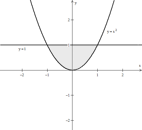
Find intervals of integration for dydx over the shaded region and set up the double integral.

To set up the integral pay close attendtion to the order of the differentials, dy and dx.
Since dy is prior to dx we set up the integral so that we first cover the intervals for y and then those for x. That is, the intervals of y are a function of x.
Our shaded region is the area between the curves y = x² and y = 1. Hence x² ≤ y ≤ 1. Note that this area runs from - 1 ≤ x ≤ 1.

Thus our intervals of integration yield the double integral ∫_{− 1}¹ ∫_x²¹ f dydx. Note the order of integration corresponds to the opposite order of the differentials.

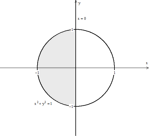
Find intervals of integration for dxdy over the shaded region and set up the double integral.

To set up the integral pay close attendtion to the order of the differentials, dy and dx.
Since dx is prior to dy we set up the integral so that we first cover the intervals for x and then those for y. That is, the intervals of x are a function of y.
Our shaded region is the left side of the circle x² + y² = 1. Solving for x yields x = ±√{1 − y²} , we only want the left side, so we take the negative result.
Hence − √{1 − y²} ≤ x ≤ 0 and this area runs from − 1 ≤ y ≤ 1.

Thus our intervals of integration yield the double integral ∫_{− 1}¹ ∫_{− √{1 − y²}}⁰ f dxdy. Note the order of integration corresponds to the opposite order of the differentials.

i) Integrate ∫_{− 2}¹ 5xy dy.

Taking the integral in respect to y takes any other variable as a constant.

So ∫_{− 2}¹ 5xy dy = [5/2]xy² |_{− 2}¹ = [5/2]x(1)² − [5/2]x( − 2)² = [5/2]x − 10x = − [15/2]x.

ii) Integrate ∫₁³ 5xy dx.

Taking the integral in respect to x takes any other variable as a constant.

So ∫₁³ 5xy dx = [5/2]x²y |₁³ = [5/2](3)²y − [5/2](1)²y = [45/2]y − [5/2]y = 20x

iii) Integrate ∫₁³ ∫_{− 2}¹ 5xy dydx.

We take the integral in respect to the order of the differentials.

So ∫₁³ ∫_{− 2}¹ 5xy dydx = ∫₁³− [15/2]x dx = − [15/4]x² |₁³ = − [15/4]( 9 − 1 ) = − 30

iv) Integrate ∫_{− 2}¹ ∫₁³ 5xy dxdy.

We take the integral in respect to the order of the differentials.

So ∫_{− 2}¹ ∫₁³ 5xy dxdy = ∫_{− 2}¹ 20x dy = 10x² |_{− 2}¹ = 10( 1 − 4 ) = − 30. Note that ∫₁³ ∫_{− 2}¹ 5xy dydx = ∫_{− 2}¹ ∫₁³ 5xy dxdy.

i) Integrate ∫_{− 2}⁰ cos(x) dy.

Taking the integral in respect to y takes any other variable as a constant.

So ∫_{− 2}⁰ cos(x) dy = |ycos(x) |_{− 2}⁰ = (0)(cos(x)) − ( − 2)cos(x) = 2cos(x)

ii) Integrate ∫_{− π\protect\mathord/ \protect phantom π2/ 2}⁰ e^y dx.

Taking the integral in respect to x takes any other variable as a constant.

So ∫_{− π\mathord/ \protect phantom π2 2}⁰ e^y dx = xe^y |_{− π\mathord/ \protect phantom π2 2}⁰ = (0)e^y − ( − [(π)/2] )e^y = [(πe^y)/2]

iii) Integrate ∫_{− π\mathord/ \protect phantom π2 2}⁰ ∫_{− 2}⁰ e^ycos(x) dydx.

We take the integral in respect to the order of the differentials.

So ∫_{− π\mathord/ \protect phantom π2 2}⁰ ∫_{− 2}⁰ e^ycos(x) dydx = ∫_{− π\mathord/ \protect phantom π2 2}⁰ ( e^ycos(x) |_{− 2}⁰ ) dx = ∫_{− π\mathord/ \protect phantom π2 2}⁰ ( cos(x) − e^{− 2}cos(x) ) dx = sin(x) |_{− π\mathord/ \protect phantom π2 2}⁰ − e^{− 2}sin(x) |_{− π\mathord/ \protect phantom π2 2}⁰ = 1 − e^{− 2}

iv) Integrate ∫_{− 2}⁰ ∫_{− π\mathord/ \protect phantom π2 2}⁰ e^ycos(x) dxdy.

We take the integral in respect to the order of the differentials.

So ∫_{− 2}⁰ ∫_{− π\mathord/ \protect phantom π2 2}⁰ e^ycos(x) dxdy = ∫_{− 2}⁰ ( e^ysin(x) |_{− π\mathord/ \protect phantom π2 2}⁰ ) dy = ∫_{− 2}⁰ e^y dy = e^y |_{− 2}⁰ = 1 − e^{− 2}. Note that ∫_{− π\mathord/ \protect phantom π2 2}⁰ ∫_{− 2}⁰ e^ycos(x) dydx = ∫_{− 2}⁰ ∫_{− π\mathord/ \protect phantom π2 2}⁰ e^ycos(x) dxdy.

Integrate given that y ∈ [ − 1,1], x ∈ [0,2] and f(x,y) = [1/2]xy³.

We set up our double integral in respect to the differentials dy and dx. Note that we have dydx.
So our double integral has the intervals of x followed by those of y. Then

Integrating yields ∫₀² ∫_{− 1}¹ [1/2]xy³ dydx = ∫₀² ( [1/8]xy⁴ |_{− 1}¹ ) dx = ∫₀² 0dx = 0

Integrate given that y ∈ [0,π], x ∈ [ − π,π] and g(x,y) = cos(x)sin(y).

We set up our double integral in respect to the differentials dy and dx. Note that we have dydx.
So our double integral has the intervals of x followed by those of y. Then

Integrating yields ∫_{− π}^π ∫₀^π cos(x)sin(y) dydx = ∫_{− π}^π ( − cos(x)cos(y) |₀^π ) dx = ∫_{− π}^π 2cos(x)dx = 2sin(x) |_{− π}^π = 0

Integrate given that x ∈ [ − [1/2],[1/2] ], y ∈ [0,5] and h(x,y) = ye^x.

We set up our double integral in respect to the differentials dy and dx. Note that we have dydx.
So our double integral has the intervals of x followed by those of y. Then

Integrating yields ∫_{− 1 \mathord/ \protect phantom 1 2 2}^{1 \mathord/ \protect phantom 1 2 2} ∫₀⁵ ye^x dydx = ∫_{− 1 \mathord/ \protect phantom 1 2 2}^{1 \mathord/ \protect phantom 1 2 2} ( [1/2]y²e^x |₀⁵ ) dx = ∫_{− 1 \mathord/ \protect phantom 1 2 2}^{1 \mathord/ \protect phantom 1 2 2} ( [25/2]e^x )dx = [25/2]e^x |_{− 1 \mathord/ \protect phantom 1 2 2}^{1 \mathord/ \protect phantom 1 2 2} = [25/2]( e^{1 \mathord/ \protect phantom 1 2 2} − e^{− 1 \mathord/ \protect phantom 1 2 2} )

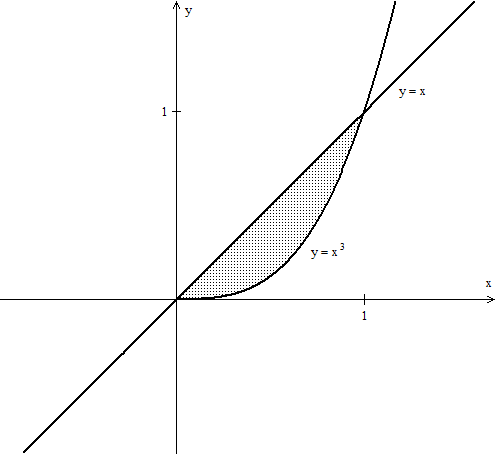
Let f(x,y) = [y/(x²)] and R be the shaded region described by:

Find dA.

Note that dA is the area covered by the differentials dx and dy. We shall integrate in respect to that order, that is dxdy.
Our region is the area between the curve y = x³ and y = x. The intervals of integration for y ∈ [x³,x].
To find the intervals of integration for x, we note that x runs from 0 to 1 along our shaded region and so x ∈ [0,1].

Then dA = ∫₀¹ ∫_x³^x [y/(x²)]dydx = ∫₀¹ ( [(y²)/(2x²)] |_x³^x ) dx = ∫₀¹ ( [((x)²)/(2x²)] − [((x³)²)/(2x²)] ) dx = ∫₀¹ ( [1/2] − [(x⁴)/2] )dx = ( [1/2]x − [1/10]x⁵ ) |₀¹ = [2/5]

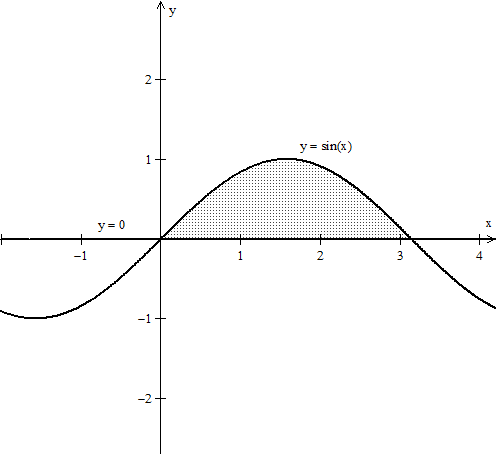
Let f(x,y) = k where k a constant, k > 0 and R be the shaded region described by:

Find dA.

Note that dA is the area covered by the differentials dx and dy. We shall integrate in respect to that order, that is dxdy.
Our region is the area between the curve y = 0 and y = sin(x). The intervals of integration for y ∈ [0,sin(x)].
To find the intervals of integration for x, we note that x runs from 0 to p along our shaded region and so x ∈ [0,p].

Then dA = ∫₀^p ∫₀^sin(x) kdydx = ∫₀^p ( ky |₀^sin(x) ) dx = ∫₀^p ( ksin(x) − ksin(0) ) dx = ∫₀^p ksin(x)dx = − kcos(x) |₀^p = 2k

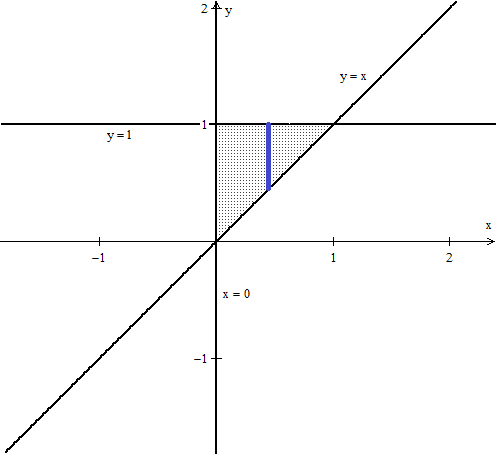
Let f(x,y) = − 2x³y² and R be the region bounded by x = 0, y = 1 and y = x.
i) Find dydx. Do not integrate.

Sketching our region yields
Note the blue line demonstrating our intervals of integration for y, that is y ∈ [x,1]. We can also see that x ∈ [0,1].

Hence dydx = ∫₀¹ ∫_x¹− 2x³y² dydx.

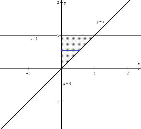
Let f(x,y) = − 2x³y² and R be the region bounded by x = 0, y = 1 and y = x.
ii) Find dxdy. Do not integrate.

Sketching our region yields
Note the blue line demonstrating our intervals of integration for x, that is x ∈ [0,y]. We can also see that y ∈ [0,1].

Hence dydx = ∫₀¹ ∫₀^y− 2x³y² dxdy.

Let f(x,y) = − 2x³y² and R be the region bounded by x = 0, y = 1 and y = x.
iii) Verify that ∫₀¹ ∫_x¹− 2x³y² dydx = ∫₀¹ ∫₀^y− 2x³y² dxdy .

We integrate each side of the equation and see if they are equal.
First ∫₀¹ ∫_x¹− 2x³y² dydx = ∫₀¹ ( − [2/3]x³y³ |_x¹ )dx = ∫₀¹ ( − [2/3]x³ + [2/3]x⁶ ) dx = ( − [1/6]x⁴ + [2/21]x⁷ ) |₀¹ = − [1/14]
Second ∫₀¹ ∫₀^y− 2x³y² dxdy = ∫₀¹ ( − [1/2]x⁴y² |₀^y )dy = ∫₀¹ ( − [1/2]y⁶ ) dy = − [1/14]y⁷ |₀¹ = − [1/14]

Since both double integrals yielded the same value, then ∫₀¹ ∫_x¹− 2x³y² dydx = ∫₀¹ ∫₀^y− 2x³y² dxdy . Note that the second double integral was simpler to compute.

« Previous Question | Next Question »

*These practice questions are only helpful when you work on them offline on a piece of paper and then use the solution steps function to check your answer.

Answer

Double Integrals

Lecture Slides are screen-captured images of important points in the lecture. Students can download and print out these lecture slide images to do practice problems as well as take notes while watching the lecture.

Intro

Double Integrals

Intro 0:00
Double Integrals 0:52

Introduction to Double Integrals
Function with Two Variables
Example 1: Find the Integral of xy³ over the Region x ϵ[1,2] & y ϵ[4,6]
Example 2: f(x,y) = x²y & R be the Region Such That x ϵ[2,3] & x² ≤ y ≤ x³
Example 3: f(x,y) = 4xy over the Region Bounded by y= 0, y= x, and y= -x+3

Multivariable Calculus

Section 1: Vectors
	Points & Vectors	28:23
	Scalar Product & Norm	30:25
	More on Vectors & Norms	38:18
	Inequalities & Parametric Lines	33:19
	Planes	29:59
	More on Planes	34:18
Section 2: Differentiation of Vectors
	Maps, Curves & Parameterizations	29:48
	Differentiation of Vectors	39:40
Section 3: Functions of Several Variables
	Functions of Several Variable	29:31
	Partial Derivatives	23:31
	Higher and Mixed Partial Derivatives	30:48
Section 4: Chain Rule and The Gradient
	The Chain Rule	28:03
	Tangent Plane	42:25
	Further Examples with Gradients & Tangents	47:11
	Directional Derivative	41:22
	A Unified View of Derivatives for Mappings	39:41
Section 5: Maxima and Minima
	Maxima & Minima	36:41
	Further Examples with Extrema	32:48
	Lagrange Multipliers	32:32
	More Lagrange Multiplier Examples	27:42
	Lagrange Multipliers, Continued	31:47
Section 6: Line Integrals and Potential Functions
	Line Integrals	36:08
	More on Line Integrals	28:04
	Line Integrals, Part 3	29:30
	Potential Functions	40:19
	Potential Functions, Continued	31:45
	Potential Functions, Conclusion & Summary	28:22
Section 7: Double Integrals
	Double Integrals	29:46
	Polar Coordinates	36:17
	Green's Theorem	38:01
	Divergence & Curl of a Vector Field	37:16
	Divergence & Curl, Continued	33:07
	Final Comments on Divergence & Curl	16:49
Section 8: Triple Integrals
	Triple Integrals	27:24
	Cylindrical & Spherical Coordinates	35:33
Section 9: Surface Integrals and Stokes' Theorem
	Parameterizing Surfaces & Cross Product	41:29
	Tangent Plane & Normal Vector to a Surface	37:06
	Surface Area	32:48
	Surface Integrals	46:52
	Divergence & Curl in 3-Space	23:40
	Divergence Theorem in 3-Space	34:12
	Stokes' Theorem, Part 1	22:01
	Stokes' Theorem, Part 2	20:32

Transcription: Double Integrals

Hello and welcome back to educator.com and multivariable calculus.0000

Today we are going to start on a new topic. We are going to be talking about double integrals.0004

The nice thing about this particular topic is you do not have to learn anything new.0008

There is going to be some new notation, but in face the notation itself is not even new. It is exactly the same as what you saw in single variable calculus, just picked up from another dimension -- dimension 1, dimension 2.0012

So for all practical purposes, you have done this stuff that we are going to be doing over and over and over again.0025

Rather than belabor the point with a lot of theory, I am actually just going to give a couple of quick definitions, and then we are just going to launch right into examples.0032

We just want to be able to handle these problems and not worry about what is going on behind the scenes too much.0041

You already know a lot of what is going on. Okay. Let us just jump right on in.0048

Okay. Now, in single variable calculus what we did was we defined this integral of f(x)/some interval from a to b.0054

We had something that looked like this... the integral from a to b of f(x) dx, and this was some number and we learned a bunch of techniques for evaluating this.0063

Well, let us go ahead and talk about what some of these things mean.0077

This right here is just a value of f at a given x on the particular interval, and this ab is of course the closed interval from a to b, just something like this.0080

If there is some function, this is a, this is b, this is the function, so we are just integrating along that length. That is the important part, we are just integrating along a length.0095

Now, this dx here it is just a differential length element -- a differential is just a fancy word for small -- so differential length element, and this symbol right here... that is just the symbol for an infinite sum.0105

So, what we have done is we have a particular function, we have a bunch of x's in between a and b, we evaluate them at each of those x's, and then we multiply by the actual length, some length element along x and then we take these numbers that we get and we just add them up with this fancy technique called integration.0137

Then we get some number. That is the integral, that is all we have done.0159

Well, we can do the same thing with a function of two variables, except now, a function of 2 variables is not defined just over the x axis, it is defined over x and y.0162

So, instead of a differential length element, what you are going to have is a differential area element.0173

Because again, now you are going to have an interval from a to b along x, but you are also going to have an interval c to d along y, so now we are going to basically break up the a to b the way we did before in single variable calculus, but we are also going to break up c to d and what you end up having is a bunch of little rectangles.0180

Instead of integrating over a length, we are integrating over a length and another length.0205

Well, length × length is area, so we are integrating over the entire area. Everything else is exactly the same, the notation is exactly the same.0212

Let us go ahead and write this out. So, for a function of two variables, f(x,y), we can integrate this function over an area, which is just length × length.0220

You will see in a minute that is exactly what you are going to be doing. You are just going to be doing one integral at a time, in an iterated fashion, in a row.0272

The symbol for it is exactly the same, except you are going to use two integral signs instead of one.0282

So, double integral, f(x,y) dy dx.0288

Also written as double integral of f, I will leave off the x,y, da.0299

dy × dx, well, differential can be x, differential in the y-direction, that gives me a little bit of a square, so this square is a differential area element. That is why we have da for dy/dx, that is it.0310

This is the one that we want to concentrate on, but you will see this when you see certain theorems, certain statements along as you understand what is happening.0327

This is a symbolic definition, so let us talk about what these mean. This is the value of f at the point (x,y).0337

This is a differential area element.0349

So, instead of having a very, very, tiny length, like single variable calculus, what we have is a really, really tiny area. One of these small rectangles or squares.0356

This, of course, is the symbol for the infinite sum -- the symbol for infinite sum -- and we use two of them to differentiate from the single variable because we are talking about two variables.0367

Later, when we do functions of three variables, you are going to see triple integral, three integral signs. It actually exists that you can keep going.0382

Okay, that is it. That is literally all that is going on here.0391

Let me go ahead and draw out one more time this thing just to make sure we completely understand.0396

So, now, because our domain is now in two dimensions, we are going to split up the x length, we are going to split up the y length, and we are just going to add the value of the function over all of these little rectangles, that is what this is.0405

Now, I am going to write out how we actually evaluate this. The practical way of finding the integral, and we do it with a single integral at a time.0423

So, let us go here. The double integral of f(x,y) dy/dx, is evaluated as -- let me go ahead and write over here -- so from a to b, from c to d, so, our interval along the x-axis is a to b, our interval along the y axis is c to d.0434

It is equivalent to taking the integral from a to b, taking the integral from c to d of f(x,y) dy, and then dx.0478

What this symbol means is that we are going to be working from the inside out, just like we do in mathematics.0495

What we are going to do is we are going back to one variable first, in this particular case, dy, f(x,y) dy, and when we do this we have to remember that y is the variable we are integrating with respect to so we keep x constant.0500

When we do this, and we evaluate this integral from c to d, we are going to get a function x.0515

Now this function of x is what we integrate from a to b and we get our final answer. That is it, this is called iterated integration and you can actually do the integral in either order.0519

You can either do f(x,y) dy dx, or you can do f(x,y) dx dy.0531

The problem itself, the particular domain you are going to be working with, will decide for you which you are going to integrate first.0536

Again, you are just integrating one variable at a time. let us just go ahead and jump into some examples, and hopefully it will all make sense.0544

Again, you have done this over and over and over again. Now instead of just stopping after one integral, you are doing another integral after that. The only thing that you have to watch out for is keeping track of the variables.0553

If you are going to be integrating with respect to y, make sure to keep x constant and carry it forward.0563

If you are integrating with respect to x, hold y constant, and carry it forward and do the evaluation. That is actually going to be the biggest stumbling block in this. It is not going to be the mathematics itself, it is going to be keeping track of what is going on.0571

So, example 1. Find the integral of xy³ over the region x goes from 1 to 2, and y goes from 4 to 6.0585

We have this little bit of a rectangle, we have 1, we have 2, let us say 4 is here. Let us say 6 is here, so we have this little rectangle that we are going to be evaluating this function, integrating this function over this domain.0622

Well, the integral, I will just call it i. In this particular case I have a choice since I am given the endpoints of the intervals explicitly, I can do dx dy, or I can do dy dx.0642

I am going to do dy first and save dx for last. Personal choice.0657

So I am going to integrate from 1 to 2. I am going to integrate from 4 to 6 -- we are working inside out -- xy³ dy dx.0660

okay. So, I am going to do the first integral. The inside integral first. This is going to equal the integral from 1 to 2, and it is always great to write out everything, do not keep things in your head, do not write things shorthand, write everything out.0672

It is not going to hurt if you have a couple of extra lines of mathematics, at least that way if there is a problem, you can follow it -- working your way back.0686

Now, when you integrate this, this symbol stays, we are doing this integration. We are integration with respect to y, x stays constant.0696

Well, integrate y³, the integral of y³ is y⁴/4, so it becomes xy⁴/4 evaluated from 4 to 6 and then dx... so far so good.0705

That equals the integral from 1 to 2, well when I put 6 into y and evaluate this, I am going to end up with so 6⁴/4.0721

I get the integral of 324x -... and of course I put 4 in for y, take the fourth power, divide by 4, multiply by 6, I am going to get -64x dx.0736

That is equal to the integral from 1 to 2 of 260x dx.0752

I am going to pull the 260 out because that is just my personal preference. I like to keep the constants outside and multiply them at the end.0759

260, integral of x, dx = 260 × x²/2 evaluated from 1 to 2.0770

I just integrated this now with respect to x. I got x²/2, and when I run through this evaluation putting 2 in, subtracting putting 1 in, multiplying by 260, I end up with 390.0781

That is it. Nice and simple. Okay.0796

Let us go ahead and give a physical interpretation of what this means and it might help, it might not. In single variable calculus, we had some function and we had the interval from a to b. Well, we interpret the integral physically as the area underneath the graph.0801

Okay. We have the same thing in a function of two variables. We said in previous lessons that a function of two variables, since it is defined over a region in the x,y plane, the value of the function can actually be used as a third variable.0821

We can graph 3-space. Basically, a function of two variables is a surface in 3-space, so let us go ahead and draw a little -- so this is the x, and this is the y, and this is the z -- so there are some surface above the x,y plane.0836

Well, basically, the integral of a function of two variables over a particular region can be interpreted as the volume of everything above that region up to the surface. That is it.0861

Again, the area underneath the graph, the volume underneath the graph. We are just moving up one dimension. That is a physical interpretation that is there for you. If you want to think about it that way, that is fine.0884

I think it helps to -- you know -- in certain circumstances, but it is important to remember that an integral is a number. It is an algebraic property, not necessarily a physical property. It can be interpreted as such, but that is not what it is.0894

Let us go ahead and do another example here. So, example 2.0908

This time, f -- let us let f equal to x²y -- and r be the region such that x runs from 2 to 3 and y is the region that is above, well between, the functions x² and x³.0918

Let us go ahead and draw this out. Again, we do not need a precise drawing... that is the x². that is the x³, let us say this is 2 and this is 3.0962

We have that, we have that, so the region that we are looking at is that region right there. That is the area over which we are going to be integrating this particular function.0975

Okay. So, in this particular case, we are constrained by the nature of the problem to do our... to differentiate with respect to y first and then differentiate with respect to x. It is simply easier that way.0990

So, let us go ahead and do it.1005

So, the integral is equal to the integral from 2 to 3, of the integral, so the lower function is the x², the upper in this case is the x³.1008

So, we are going to go from x² to x³, this is perfectly acceptable.1023

The function that we are integrating is x²y dy dx, so we just need to make sure that we keep the order correct.1027

Well, this is going to equal the integral 2 to 3. Now when we integrate x²y with respect to y, we are holding x² constant, so it is going to be y²/2... x² y²/2.1041

We are evaluating it from x² to x³, and then we are going to do the dx.1055

This is going to be the integral from 2 to 3 -- oops, let us see if we can eliminate as many of these stray lines as possible -- the integral from 2 to 3, so when we put x³ in for here, we get x into y because we are evaluating with respect to y.1060

This is going to be x⁶ × x², so we are going to get x⁸/2 - ... and when we put x² in for here, it is going to be x⁴ × x², it is going to be x⁶/2 dx.1079

Right? So far so good. Let us go ahead and go to the next page.1099

When we do that integration, it is going to equal -- actually, let me write it again so we have it on this page -- 2 to 3 x⁸/2 - x⁶/2 dx = x⁹/18 - x⁷/14.1103

Right? 6, 7 × 2 is 14, 9 × 2 is 18. We are going to evaluate that from 2 to 3, and then when we do this evaluation we are going to end up somewhere in the neighborhood -- ahh its okay, I am just going to do an approximate... it is going to be somewhere in the neighborhood of about 918 when you actually run that.1130

The number itself, I mean it is important, but it is not that important. It is the process that is important. This is where we want to come to.1153

Now, let us go ahead and do a third example. Example 3.1163

We have f(x,y) is equal to... this time, 4xy is our function, over the region bounded by y = 0, y = x and y = -x + 3.1172

Let us go ahead and draw this region out and go ahead and see what it is we are looking at.1200

So, y = 0, that is the x axis. y = x, that is this line right here, y = -x + 3, so let us go up 3, and let us go down that way in a 45 degree angle.1207

So this is going to hit at 3 and let us go ahead and put a half-way mark here. This is actually going to be 3/2 because these have the same slope.1224

In this particular case, our region is right here, this triangle. We are going to be integrating this function over this particular triangle.1235

Of course you remember from first variable calculus, sometimes regions have to be split up simply to make the integral a little bit easier to handle.1242

In this particular case, I am going to decide to save the integration with respect to x last, the outside integral.1249

Since that is the case, I am actually going to split this into two regions. This region r, I am going to split it up into R1 and R2.1257

I am going to integrate up to here, and up to there. Then I am going to add those 2 together. The reason that I do that is the upper function from here to here is different. Here it is 0 to x, here it is 0 to -x + 3, which is why I am splitting it up.1265

Let me erase this thing. So, in this particular case, our integral over R is going to equal the integral over R1 + the integral over R2 because the integrals are additive, that is exactly right.1282

Let us go ahead and deal with the integral of -- I am going to move to the next page -- so, the integral over R1 is going to equal the integral from 0 to 3/2, that is the first half and the y value, let me draw my domain again so I have it here.1300

It is going to be that, and that, so the y value is going to go from 0 to x, and my function is 4xy dy dx.1324

That is -- excuse me -- equal to the integral from 0 to 3/2 of 2xy², I am integrating with respect to y, I am holding that constant, y²/2, the 2 and the 4 cancel leaving me 2xy², and I am evaluating that from 0 to x dx.1339

That is going to equal, well, 2 × the integral from 0 to 3/2... when I put x in for here, it is x² × x is x³, so it is x³ dx.1359

This is 0, so it goes away and now that is going to equal 2 × x⁴/4 evaluated from 0 to 3/2.1374

When I go ahead and do that, I get 81/32, so that is the integral with respect to the first region.1389

Now we will do the integral over the second region, this region right here.1399

So, the integral over region 2 is equal to -- now we are integrating from 3/2 to 3 -- so, 3/2 to 3, and the y value is going to be 0 to -x + 3.1404

Because now the upper function is -x + 3 and again our function is 4xy dy dx.1423

Well, that is going to equal 3/2 to 3, it is going to be again 2xy², evaluated from 0 to -x + 3.1432

When I put this in here, let us see if I have enough room, no I probably do not so let me come down here -- the integral from 0... nope, doing 3/2 to 3 now -- again, keep track of our numbers.1449

From 3/2 to 3, it is going to be 2x × -x + 3², because the 0 goes away and I am just putting this into that, dx.1464

Ohh... crazy... we do not want these crazy lines all over the place.1480

Okay. 0 dx, when I multiply this out, actually I am going ot multiply everything out here so it is fine. We will do 3/2 over 3, it is going to be 2x × x² - 6x + 9 dx = the integral from 3/2 to 3 of 2x³ - 12 x² + 19x dx.1490

When I go ahead and evaluate that, I use mathematical software to evaluate that, I ended up with 243 over 32, therefore the integral of f over our original region R is equal to the 81/32, the integral over the first region + 243/32, the integral of the other region = 324/32.1532

That is it. Okay. So, in this particular case, I took this region and I divided it into 2 regions and I did 2 separate integrals.1567

There is a way to actually do this as one integral by just reversing the order of integration by doing dx first and then doing the dy.1575

I will go ahead and show you what that is. I will not do the integration, but I will show you how to approach it.1584

So, let me draw the domain again. We had that, and we had this, okay? So this was 3, this was 0, we had 3/2 here, this was 3, this was y = x, or if I wrote it in terms of x, x = y.1590

Okay. This graph right here, that is the y = -x + 3. If I write it in terms of x, it is x = 3 - y.1619

Now, I am thinking about it this way. I am going to do my final integration with respect to y, which means I am going to go from 0 all the way up to 3.1630

In this particular case, there is no interference. The difference -- it says if I turn the graph this way -- the difference, this length right here, okay, that I am going to be integrating this way... this length is the difference between this function and this function.1644

In this particular case, I can go ahead and take the difference between this function and this function, and then integrate with respect to y this way, so the integral looks like this.1662

The integral from 0 to -- this is not 3, this is actually 3/2 -- 0 to, this value right here is 3/2.1681

If you solve simultaneously, this is x is 3/2, this is y is 3/2, so this y value is 3/2.1692

So 0 to 3/2, the integral... well, it is going to be... you want to keep this positive, so we are taking this function, this function, this is the lower that is the upper, so let us go 3 - y to y, 4xy, this time we are going to do dx dy.1699

That is it. So, you can do this as a single integral as long as you change your perspective and if you are integrating finally along this direction, the first integration that you do, which is going to be this way, well, this difference always stays the same in the sense that it is always going to be a difference between this function and this function.1726

That is it. The outer integral covers the entire region, I did not actually have to break this up, but the way that I chose to do it, simply because I like doing x last.1752

I had to break this region up into 2, and the reason I broke it up into 2 is because the y value is actually different depending on which function I am working with past this 3/2 mark.1764

That is it. That is our introduction to double integrals. Thank you for joining us here at educator.com, we will see you next time. Bye-bye.1778

Related Books

Multivariable Calculus by Stewart, 7th Edition

Author: James Stewart

ISBN: 538497815

Publisher: Brooks Cole

Year: 2011

The book is filled with clear and accurate descriptions of concepts and is also has many relevant, real-world examples.

Related Books

Name	Description	Link
BookRenter.com	BookRenter.com is simply the most reliable online textbook rental service.	Visit BookRenter.com
PhysicsForums.com Homework Help	Physics Forums is a scientific community for students looking for math & science help.	Visit PhysicsForums.com Homework Help

Multivariable Calculus Double Integrals

Share this knowledge with your friends!

Copy & Paste this embed code into your website’s HTML

Discussion

Answer Engine

Practice Questions

Download Lecture Slides

Table of Contents

Transcription

Related Books

Answer EngineGet answers to any question!Ask any question related to Multivariable Calculus

Double Integrals

Double Integrals

Multivariable Calculus

Transcription: Double Integrals

Related Books

Related Books

Start Learning Now

Membership Overview

Multivariable Calculus Double Integrals

Share this knowledge with your friends!

Copy & Paste this embed code into your website’s HTML

Discussion

Answer Engine

Practice Questions

Download Lecture Slides

Table of Contents

Transcription

Related Books

Answer EngineGet answers to any question!Ask any question related to Multivariable Calculus

Double Integrals

Double Integrals

Multivariable Calculus

Transcription: Double Integrals

Related Books

Related Books

Available 24/7. Unlimited Access to Our Entire Library.

Searchable Lessons

Get Answers & Community Support

Downloadable Lecture Notes

Study Guides, Worksheets and Extra Example Lessons

Start Learning Now

Membership Overview