Raffi Hovasapian

Further Examples with Gradients & Tangents

Slide Duration:

Table of Contents

Section 1: Vectors

Points & Vectors

28m 23s

Intro

0:00

Points and Vectors

1:02

A Point in a Plane

1:03

A Point in Space

3:14

Notation for a Space of a Given Space

6:34

Introduction to Vectors

9:51

Adding Vectors

14:51

Example 1

16:52

Properties of Vector Addition

18:24

Example 2

21:01

Two More Properties of Vector Addition

24:16

Multiplication of a Vector by a Constant

25:27

Scalar Product & Norm

30m 25s

Intro

0:00

Scalar Product and Norm

1:05

Introduction to Scalar Product

1:06

Example 1

3:21

Properties of Scalar Product

6:14

Definition: Orthogonal

11:41

Example 2: Orthogonal

14:19

Definition: Norm of a Vector

15:30

Example 3

19:37

Distance Between Two Vectors

22:05

Example 4

27:19

Multivariable Calculus Further Examples with Gradients & Tangents

Name: Multivariable Calculus: Further Examples with Gradients & Tangents
Brand: Educator.com
Price: 35 USD
Availability: InStock

Section 4: Chain Rule and The Gradient: Lecture 3 | 47:11 min

Lecture Description

Next Lecture

Previous Lecture

Discussion
Answer Engine
Practice Questions
Download Lecture Slides
Table of Contents
Transcription
Related Books

Lecture Comments (13)

	0 answers Post by Brett Pienaar on October 28 at 08:53:03 AM you would think this organization would keep a decent book mark as to where the student last left off instead of waffling on and on...
	1 answer Last reply by: Professor Hovasapian Tue Oct 16, 2018 10:53 PM Post by Mohamed Talni on October 15, 2018 Dear Professor Hovasapian, I really enjoy your explanation and insight. I have a question that I do not understand: Consider the first quadrant in the OXY plane in R2. Point O is the origin and the points P and Q are chosen on the y-axis and the x-axis, respectively as it is showed in the figure below. We create a family of line segments like PQ in a way that OP+OQ=10 1. Determine the equation of the curve which appears by drawing more and more such line segments. 2. Suppose we want to investigate a similar problem in the three dimensional case. Consider the first octant of the OXYZ in R3. Then we create a family of plane segments such that OP+OQ+OR=10. Then what would be the equation of the surface which will arise by drawing infinitely many such planes.
	1 answer Last reply by: Professor Hovasapian Mon Oct 13, 2014 6:32 PM Post by sam sohirad on October 11, 2014 hi raffi for example 1, can we use the cross product to find a vector in the direction of the space curve (intersection curve of the planes)? I dont know if my thought process is correct but as i understood the two planes intersect and then we have a curve of intersection. we are looking for the tangent line at a point on this curve. in order to find the equation of a line we need 2 things; 1 a point on the line (3,2,-6) and a vector pointing in the direction of this line. since the 2 surfaces meet and create a curve, we can find the gradient vector at a certain point on the line. this will give us 2 normal vectors at a certain point of intersection. we can then go on to find the cross product of these 2 normal vectors at a mutual point to find a perpendicular vector at this point, thereby giving us the direction of the line. we then plug into our equation X=tv+P and have the vector equation of a line at the point. if i use this method will i get the equation of a line that touches the point (3,2,-6)making it an equation of a tangent line? i also understand what you said about the planes and when they intersect we get a line and that is the equation of our tangent line at that point, but i dont see how we used the planes in example 1? to me it seems we found the gradients of the surfaces.
	5 answers Last reply by: Josh Winfield Sat May 11, 2013 8:07 AM Post by Josh Winfield on February 12, 2013 Example 2:You ask to find c'(t) but found c'(0) instead. Which one where we supposed to find? Example 3: âˆš(152) x âˆš(149) = 150.5 not -150.5 So the angle you get arccos(-150/150.5) = 175.33 (degrees)
	1 answer Last reply by: Professor Hovasapian Thu Sep 6, 2012 2:43 PM Post by Ian Vaagenes on September 6, 2012 Great course Raffi, you have a real gift for making things understandable. Any chance you'll do a few lectures on measure theory/probability theory?

Answer EngineGet answers to any question!Ask any question related to Multivariable Calculus

Working on the solution...

Further Examples with Gradients & Tangents

Find the parametric representation for a line tangent to the curve of intersection of the two surfaces
[(x²)/4] + y² + [(z²)/9] = 3 and y² + z² = 10 at (2, − 1,3).

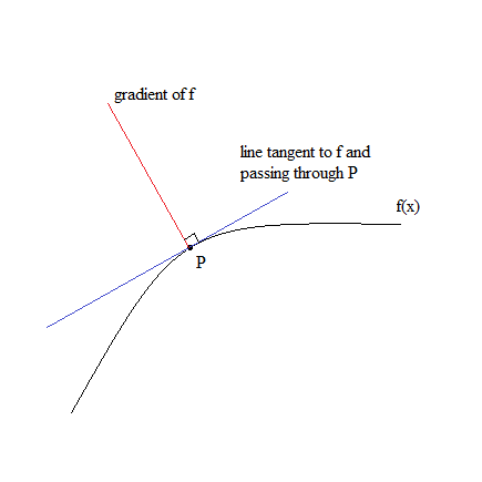
Recall that the gradient of a function at a point →P is a vector perpendicular to the line tangent to the function passing through →P. See image.
Let f(x,y,z) = [(x²)/4] + y² + [(z²)/9] − 3 and g(x,y,z) = y² + z² − 10. By finding ∇f(2, − 1,3) and ∇g(2, − 1,3) we can obtain a vector →v passing through →P and perpendicular to both ∇f(2, − 1,3) and ∇g(2, − 1,3).
Now, ∇f(x,y,z) = ( [x/2],2y,[2z/9] ) and ∇g(x,y,z) = (0,2y,2z). Hence ∇f(2, − 1,3) = ( 1, − 2,[2/3] ) and ∇g(2, − 1,3) = (0, − 2,6).
Let →v = (v₁,v₂,v₃), since ∇f(2, − 1,3) and →v are prependicular we have ∇f(2, − 1,3) ×→v = 0. So ∇f(2, − 1,3) ×(v₁,v₂,v₃) = ( 1, − 2,[2/3] ) ×(v₁,v₂,v₃) = v₁ − 2v₂ + [2/3]v₃ = 0.
Similarly ∇g(2, − 1,3) ×→v = 0. So ∇g(2, − 1,3) ×(v₁,v₂,v₃) = (0, − 2,6) ×(v₁,v₂,v₃) = − 2v₂ + 6v₃ = 0.
We now have a system of equations
v₁ − 2v₂ + [2/3]v₃ = 0
− 2v₂ + 6v₃ = 0
which yield
v₁ = [16/3]v₃
v₂ = 3v₃
v₃ = k
where k > 0 is a constant.
Setting v₃ = 3 we obtain v₂ = 9 and v₁ = 16. Our vector →v = (16,9,3). Note that the value of v₃ is arbitrary.
This vector →v has the same direction of the line tangent to the curve of intersection between the surfaces [(x²)/4] + y² + [(z²)/9] = 3 and y² + z² = 10 at (2, − 1,3).
Hence we can construct a parametric representation of the line using →x(t) = →P + t→v.
Substituting yields →x(t) = →P + t→v = (2, − 1,3) + t(16,9,3).

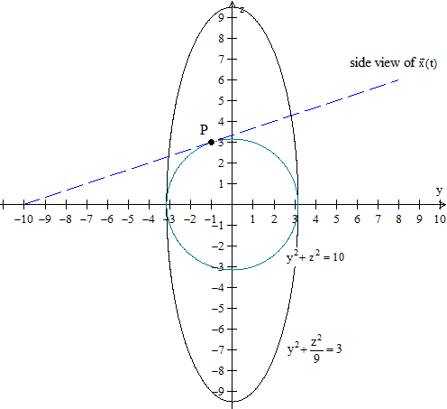
To have a better understanding, note that [(x²)/4] + y² + [(z²)/9] = 3 is an ellipsoid and y² + z² = 10 is a cylinder along the x - axis. The image below depicts the yz - plane view of our surfaces. Where would the curves of intersection be?

Find the parametric representation for a line tangent to the curve of intersection of the two surfaces√{6z − x² − y²} = 3 and 4x² + y² + z = 5 at (0,√3 ,2).

Recall that the gradient of a function at a point →P is a vector perpendicular to the line tangent to the function passing through →P. See image.
Let f(x,y,z) = √{6z − x² − y²} − 3 and g(x,y,z) = 4x² + y² + z − 5. By finding ∇f(0,√3 ,2) and ∇g(0,√3 ,2) we can obtain a vector →v passing through →P and perpendicular to both ∇f(0,√3 ,2) and ∇g(0,√3 ,2).
Now, ∇f(x,y,z) = ( [( − x)/(√{6z − x² − y²} )],[( − y)/(√{6z − x² − y²} )],[3/(√{6z − x² − y²} )] ) and ∇g(x,y,z) = (8x,2y,1). Hence ∇f(0,√3 ,2) = ( 0, − [(√3 )/3],1 ) and ∇g(0,√3 ,2) = (0,2√3 ,1).
Let →v = (v₁,v₂,v₃), since ∇f(0,√3 ,2) and →v are prependicular we have ∇f(0,√3 ,2) ×→v = 0. So ∇f(0,√3 ,2) ×(v₁,v₂,v₃) = ( 0, − [(√3 )/3],1 ) ×(v₁,v₂,v₃) = − [(√3 )/3]v₂ + v₃ = 0.
Similarly ∇g(0,√3 ,2) ×→v = 0. So ∇g(0,√3 ,2) ×(v₁,v₂,v₃) = (0,2√3 ,1) ×(v₁,v₂,v₃) = 2√3 v₂ + v₃ = 0.
We now have a system of equations
− [(√3 )/3]v₂ + v₃ = 0
2√3 v₂ + v₃ = 0
which yield
v₁ = k
v₂ = 0
v₃ = 0
where k > 0 is a constant.
Setting v₁ = 1 our vector →v = (1,0,0). Note that the value of v₁ is arbitrary.
This vector →v has the same direction of the line tangent to the curve of intersection between the surfaces √{6z − x² − y²} = 3 and 4x² + y² + z = 5 at (0,√3 ,2).
Hence we can construct a parametric representation of the line using →x(t) = →P + t→v.

Substituting yields →x(t) = →P + t→v = (0,√3 ,2) + t(1,0,0) = (t,√3 ,2).

Find the parametric representation for a line tangent to the curve of intersection of the two surfacesx² − y² + z² = 4 and 9x² − 4y² + z² = 9 at (1,1,2).

Recall that the gradient of a function at a point →P is a vector perpendicular to the line tangent to the function passing through →P. See image.
Let f(x,y,z) = x² − y² + z² − 4 and g(x,y,z) = 9x² − 4y² + z² − 9. By finding ∇f(1,1,2) and ∇(1,1,2) we can obtain a vector →v passing through →P and perpendicular to both ∇f(1,1,2) and ∇g(1,1,2).
Now, ∇f(x,y,z) = ( 2x, − 2y,2z ) and ∇g(x,y,z) = (18x, − 8y,2z). Hence ∇f(1,1,2) = ( 2, − 2,4 ) and ∇g(1,1,2) = (18, − 8,4).
Let →v = (v₁,v₂,v₃), since ∇f(1,1,2) and →v are prependicular we have ∇f(1,1,2) ×→v = 0. So ∇f(1,1,2) ×(v₁,v₂,v₃) = ( 2, − 2,4 ) ×(v₁,v₂,v₃) = 2v₁ − 2v₂ + 4v₃ = 0.
Similarly ∇g(1,1,2) ×→v = 0. So ∇g(1,1,2) ×(v₁,v₂,v₃) = (18, − 8,4) ×(v₁,v₂,v₃) = 18v₁ − 8v₂ + 4v₃ = 0.
We now have a system of equations
2v₁ − 2v₂ + 4v₃ = 0
18v₁ − 8v₂ + 4v₃ = 0
which yield
v₁ = [3/8]v₂
v₂ = k
v₃ = 0
where k > 0 is a constant.
Setting v₂ = 8 we obtain v₁ = 3 and v₃ = 0. Our vector →v = (3,8,0). Note that the value of v₂ is arbitrary.
This vector →v has the same direction of the line tangent to the curve of intersection between the surfaces x² − y² + z² = 4 and 9x² − 4y² + z² = 9 at (1,1,2).
Hence we can construct a parametric representation of the line using →x(t) = →P + t→v.

Substituting yields →x(t) = →P + t→v = (1,1,2) + t(3,8,0).

Let f(x,y) = 2x² − xy, g(x,y) = y² − x² and C(0) = (1,1).
Suppose [d/dt]f(C(0)) = 2 and [d/dt]g(C(t)) = − 3. Find C′(0).

Recall that [d/dt]F(C(t)) = ∇F(C(t)) ×C′(t). We can find the gradients of both f and g and use our available information to solve for C′(t).
Now, ∇f(x,y) = (4x − y, − x) and ∇g(x,y) = ( − 2x,2y). Note that since C(0) = (1,1) we can compute ∇f(C(0)) and ∇g(C(0)) by letting x = 1 and y = 1.
We now obtain a system of equations
[d/dt]f(C(0)) = ∇f(C(0)) ×C′(0)
[d/dt]g(C(0)) = ∇g(C(0)) ×C′(0)
or by substitution
2 = (3, − 1) ×(u,v)
− 3 = ( − 2,2) ×(u,v)
where C′(0) = (u,v).
Simplifying yields
2 = 3u − v
− 3 = − 2u + 2v
which has solutions u = [1/4] and v = − [5/4].

Hence C′(0) = ( [1/4], − [5/4] ).

Let f(x,y) = cos(x + y) − sin(y), g(x,y) = sin(xy) and C(p) = ( 0, − [3p/2] ). Suppose [d/dt]f(C(p)) = − [1/2] and [d/dt]g(C(p)) = [2/5]. Find C′(p).

Recall that [d/dt]F(C(t)) = ∇F(C(t)) ×C′(t). We can find the gradients of both f and g and use our available information to solve for C′(t).
Now, ∇f(x,y) = ( − sin(x + y), − sin(x + y) − cos(y)) and ∇g(x,y) = (ycos(xy),xcos(xy)). Note that since C(p) = ( 0, − [3p/2] ) we can compute ∇f(C(p)) and ∇g(C(p)) by letting x = 0 and y = − [3p/2].
We now obtain a system of equations
[d/dt]f(C(p)) = ∇f(C(p)) ×C′(p)
[d/dt]g(C(p)) = ∇g(C(p)) ×C′(p)
or by substitution
− [1/2] = (1,1) ×(u,v)
[2/5] = ( − [3p/2],0 ) ×(u,v)
where C′(p) = (u,v).
Simplifying yields
− [1/2] = u + v
[2/5] = − [3p/2]u
which has solutions u = − [4/15p] and v = − [1/2] + [4/15p].

Hence C′(p) = ( − [4/15p], − [1/2] + [4/15p] ).

Let f(x,y) = √{x − 1} + √{y − 1} , g(x,y) = √{xy} and C(1) = ( 2,5 ). Suppose [d/dt]f(C(1)) = 4 and [d/dt]g(C(1)) = − 2. Find C′(1).

Recall that [d/dt]F(C(t)) = ∇F(C(t)) ×C′(t). We can find the gradients of both f and g and use our available information to solve for C′(t).
Now, ∇f(x,y) = ( [1/(2√{x − 1} )],[1/(2√{y − 1} )] ) and ∇g(x,y) = ( [y/(2√{xy} )],[x/(2√{xy} )] ). Note that since C(1) = ( 2,5 ) we can compute ∇f(C(1)) and ∇g(C(1)) by letting x = 2 and y = 5.
We now obtain a system of equations
[d/dt]f(C(1)) = ∇f(C(1)) ×C′(1)
[d/dt]g(C(1)) = ∇g(C(1)) ×C′(1)
or by substitution
4 = ( [1/2],[1/4] ) ×(u,v)
− 2 = ( [5/(2√{10} )],[1/(√{10} )] ) ×(u,v)
where C′(1) = (u,v).
Simplifying yields
4 = [1/2]u + [1/4]v
− 2 = [5/(2√{10} )]u + [1/(√{10} )]v
which has solutions u = − 32 − 4√{10} and v = 80 + 8√{10} .

Hence C′(1) = ( − 32 − 4√{10} ,80 + 8√{10} ).

Let f(x,y) = e^{2x − 3y}, g(x,y) = xe^{− y²} and C( − 1) = ( − 1,1). Suppose [d/dt]f(C( − 1)) = 7 and [d/dt]g(C( − 1)) = 12. Find C′( − 1).

Recall that [d/dt]F(C(t)) = ∇F(C(t)) ×C′(t). We can find the gradients of both f and g and use our available information to solve for C′(t).
Now, ∇f(x,y) = (2e^{2x − 3y}, − 3e^{2x − 3y}) and ∇g(x,y) = (e^{− y²}, − 2xye^{− y²}). Note that since C( − 1) = ( − 1,1) we can compute ∇f(C( − 1)) and ∇g(C( − 1)) by letting x = − 1 and y = 1.
We now obtain a system of equations
[d/dt]f(C( − 1)) = ∇f(C( − 1)) ×C′( − 1)
[d/dt]g(C( − 1)) = ∇g(C( − 1)) ×C′( − 1)
or by substitution
7 = (2e^{− 5}, − 3e^{− 5}) ×(u,v)
12 = (e^{− 1},2e^{− 1}) ×(u,v)
where C′( − 1) = (u,v).
Simplifying yields
7 = 2e^{− 5}u − 3e^{− 5}v
12 = e^{− 1}u + 2e^{− 1}v
which has solutions u = [36/7]e + 2e⁵ and v = [24/7]e − e⁵.

Hence C′( − 1) = ( [36/7]e + 2e⁵,[24/7]e − e⁵ ).

Find the angle θ between the the surfaces x² + 2z² − 6x − y = − 2 and x² + 4z² − y = 6 at (1, − 1,1).

To find the angle θ between two surfaces, it suffices to find the normal vectors N₁ and N₂ to the surfaces at the point and apply cos θ = [(N₁ ×N₂)/(|| N₁ |||| N₂ ||)].
Recall that ∇F is the normal vector to a surface at a point P. Let f(x,y,z) = x² + 2z² − 6x − y + 2 and g(x,y,z) = x² + 4z² − y − 6.
Then ∇f(x,y,z) = (2x − 6, − 1,4z) and ∇g(x,y,z) = (2x, − 1,8z), so that N₁ = ∇f(1, − 1,1) = ( − 4, − 1,4) and N₂ = ∇g(1, − 1,1) = (2, − 1,8).

Hence cos θ = [(N₁ ×N₂)/(|| N₁ |||| N₂ ||)] = [(( − 4, − 1,4) ×(2, − 1,8))/(|| ( − 4, − 1,4) |||| (2, − 1,8) ||)] = [25/(3√{253} )] and so θ = cos^{− 1}( [25/(3√{253} )] ) ≈ 58.4^o

Find the angle θ between the the surfaces 3x² − 5y² − z = 9 and y² + xy − z = 5 at (2,1, − 2).

To find the angle θ between two surfaces, it suffices to find the normal vectors N₁ and N₂ to the surfaces at the point and apply cos θ = [(N₁ ×N₂)/(|| N₁ |||| N₂ ||)].
Recall that ∇F is the normal vector to a surface at a point P. Let f(x,y,z) = 3x² − 5y² − z − 9 and g(x,y,z) = y² + xy − z − 5.
Then ∇f(x,y,z) = (6x, − 10y, − 1) and ∇g(x,y,z) = (y,2y + x, − 1), so that N₁ = ∇f(2,1, − 2) = (12, − 10, − 1) and N₂ = ∇g(2,1, − 2) = (1,4, − 1).

Hence cos θ = [(N₁ ×N₂)/(|| N₁ |||| N₂ ||)] = [((12, − 10, − 1) ×(1,4, − 1))/(|| (12, − 10, − 1) |||| (1,4, − 1) ||)] = [( − 9)/(7√{10} )] and so θ = cos^{− 1}( [( − 9)/(7√{10} )] ) ≈ 114^o

Find the angle θ between the the surfaces xy² + yz² = − 3 and x + y − z² = − 6 at (1, − 3,2).

To find the angle θ between two surfaces, it suffices to find the normal vectors N₁ and N₂ to the surfaces at the point and apply cos θ = [(N₁ ×N₂)/(|| N₁ |||| N₂ ||)].
Recall that ∇F is the normal vector to a surface at a point P. Let f(x,y,z) = xy² + yz² + 3 and g(x,y,z) = x + y − z² + 6.
Then ∇f(x,y,z) = (y²,2xy + z²,2yz) and ∇g(x,y,z) = (1,1, − 2z), so that N₁ = ∇f(1, − 3,2) = (9, − 2, − 12) and N₂ = ∇g(1, − 3,2) = (1,1, − 4).

Hence cos θ = [(N₁ ×N₂)/(|| N₁ |||| N₂ ||)] = [((9, − 2, − 12) ×(1,1, − 4))/(|| (9, − 2, − 12) |||| (1,1, − 4) ||)] = [55/(3√{458} )] and so θ = cos^{− 1}( [55/(3√{458} )] ) ≈ 31.1^o

« Previous Question | Next Question »

*These practice questions are only helpful when you work on them offline on a piece of paper and then use the solution steps function to check your answer.

Answer

Further Examples with Gradients & Tangents

Lecture Slides are screen-captured images of important points in the lecture. Students can download and print out these lecture slide images to do practice problems as well as take notes while watching the lecture.

Intro

Example 1: Parametric Equation for the Line Tangent to the Curve of Two Intersecting Surfaces

Example 2: Gradients & Composite Functions

Example 3: Cos of the Angle Between the Surfaces

Intro 0:00
Example 1: Parametric Equation for the Line Tangent to the Curve of Two Intersecting Surfaces 0:41

Part 1: Question
Part 2: When Two Surfaces in ℝ3 Intersect
Part 3: Diagrams
Part 4: Solution
Part 5: Diagram of Final Answer

Example 2: Gradients & Composite Functions 26:42

Part 1: Question
Part 2: Solution

Example 3: Cos of the Angle Between the Surfaces 39:20

Part 1: Question
Part 2: Definition of Angle Between Two Surfaces
Part 3: Solution

Multivariable Calculus

Section 1: Vectors
	Points & Vectors	28:23
	Scalar Product & Norm	30:25
	More on Vectors & Norms	38:18
	Inequalities & Parametric Lines	33:19
	Planes	29:59
	More on Planes	34:18
Section 2: Differentiation of Vectors
	Maps, Curves & Parameterizations	29:48
	Differentiation of Vectors	39:40
Section 3: Functions of Several Variables
	Functions of Several Variable	29:31
	Partial Derivatives	23:31
	Higher and Mixed Partial Derivatives	30:48
Section 4: Chain Rule and The Gradient
	The Chain Rule	28:03
	Tangent Plane	42:25
	Further Examples with Gradients & Tangents	47:11
	Directional Derivative	41:22
	A Unified View of Derivatives for Mappings	39:41
Section 5: Maxima and Minima
	Maxima & Minima	36:41
	Further Examples with Extrema	32:48
	Lagrange Multipliers	32:32
	More Lagrange Multiplier Examples	27:42
	Lagrange Multipliers, Continued	31:47
Section 6: Line Integrals and Potential Functions
	Line Integrals	36:08
	More on Line Integrals	28:04
	Line Integrals, Part 3	29:30
	Potential Functions	40:19
	Potential Functions, Continued	31:45
	Potential Functions, Conclusion & Summary	28:22
Section 7: Double Integrals
	Double Integrals	29:46
	Polar Coordinates	36:17
	Green's Theorem	38:01
	Divergence & Curl of a Vector Field	37:16
	Divergence & Curl, Continued	33:07
	Final Comments on Divergence & Curl	16:49
Section 8: Triple Integrals
	Triple Integrals	27:24
	Cylindrical & Spherical Coordinates	35:33
Section 9: Surface Integrals and Stokes' Theorem
	Parameterizing Surfaces & Cross Product	41:29
	Tangent Plane & Normal Vector to a Surface	37:06
	Surface Area	32:48
	Surface Integrals	46:52
	Divergence & Curl in 3-Space	23:40
	Divergence Theorem in 3-Space	34:12
	Stokes' Theorem, Part 1	22:01
	Stokes' Theorem, Part 2	20:32

Transcription: Further Examples with Gradients & Tangents

Hello and welcome back to educator.com and multi-variable calculus.0000

The last lesson we introduced the notion of the tangent plane. I thought it would be a good idea to go ahead to go ahead and do some further examples with the concepts we have been studying recently.0004

Just more practice with gradients, and tangents, and partial derivatives and things like that just to get a better sense of what is going on.0012

Just to get a sense of the different types of problems you are actually going to run across, and to use what you know about a particular situation to reason out a problem.0022

That is it, just for practice. Before we actually move on to the next topic, which is going to be directional derivatives.0032

Let us just go ahead and jump right on with the first example. Example 10038

Now, our task is to find a parametric equation for the line to the curve of intersection of the 2 surfaces, x² + y² + z² = 49.0054

x² + y² = 13 at the point (3,2,-6).0112

Let us see if that was the right point here, yes, the point (3,2,-6).0134

So, this is more than a little more complicated than what we have done before.0150

As far as the expression of the question is concerned, and that is going to happen sometimes.0157

Do not let the expression of the question lead you to believe that it is any more complicated than anything that you have done before.0161

That is the real issue. You just stop and think about it and understand what is going on.0167

As it is we only have a handful of terms at our disposal already, we have partial derivatives, which we know how to do, hopefully at this point.0173

We have the idea of the gradient vector and we have this idea of a tangent plane or a tangent line.0180

Now, let us just sort of pull back and see what it is they are actually asking us to do.0185

Find a parametric region for the line that is tangent to the curve of intersection of the 2 surfaces.0190

Here is what is happening. I will go ahead and describe it and I will write it out so that you have it for reference.0199

You know that any time 2 planes, a plane is just a surface in 3 space, it just happens to be a very simple type of surface, it is flat.0205

You know that when 1 plane meets another plane, where they intersect, it actually forms a line, right?0213

Now if I take, instead of 2 planes that are intersecting, if I actually take 2 surfaces, that are intersecting, there point of intersection actually ends up being a curve.0223

Of course we will draw all of this out in just a minute.0234

They are asking, they are saying, I have a surface, x² + y² = 49, and I have another x² + y² = 13.0239

They are going to meet in some sort of curve in 3-space. Well, at that curve, they want you to find the equation of the tangent line that hits the point of intersection and is actually tangent to the curve itself.0245

That is what they are asking. So, let us do a little bit of discussion and then we will draw some pictures and then we will actually start the problem because this is really, really important.0263

So, I will write out everything here. When 2 surfaces in R3 intersect, their points of intersection form a curve in R3.0273

Again, we will be drawing it out in just a minute so that you can actually see it.0307

Now, here is what is important. When we form the tangent plane to surface 1, and the tangent plane to which we can do, which we already know how to do.0313

The tangent plane to surface 2 at a point where they intersect, the line of intersection of these 2 planes, of these two tangent planes is, it is the line we are looking for.0342

It is the line tangent to the curve of intersection.0394

So, before I draw it out, let me just tell you what is going on once again.0408

I have a curve, I have another curve. Where they intersect is going to be some sort of another curve.0412

Well, any point along that curve where they intersect, I can actually form a plane that is tangent to one of these surfaces, and I can form the plane that is tangent to the other surface.0417

Now I have a plane, and another plane. Those 2 planes, when they intersect, they intersect in a line. Well, because they have that point p in common, that one point.0427

The line where the 2 tangent planes intersect, that is the line that happens to be tangent to the curve of intersection. That is what we are doing.0442

We are going from the surface to the tangent plane, the intersection of the 2, that is going to be our line. This is what it looks like.0448

So, I am going to do that on the next page here.0456

Okay, so, drawings, here we go. Let me see if I can get this right.0461

So I have one surface going this way, let us just go like this, like that, like that. How is that?0467

Now I have got another surface here, so I am going to go... let us go down, let us go up like this. Let us go up here, and we will just go like that.0472

So, let me draw, let me make a little bit of an erasure here so that I can see.0489

Okay. That is what we mean. If we have one surface, and another surface, where they intersect, where they actually intersect is a curve because surfaces are curved.0502

They actually intersect at a curve. That is what is happening here.0513

Now, what I can do is I can actually form the plane that is perpendicular... the plane that is tangent... so, let us say that we have some point on there.0521

So, what we want is we want the line that is going to be tangent to that curve. That is what we are looking for.0532

Well, if I form the plane that is... so we will call this surface 2, and we will call this surface 1.0538

If I form the tangent plane at that point, just surface 2, and if I form the tangent plane to that point at surface 1, I am going to end up with 2 planes.0546

Now, let me go ahead and draw those. So, I am not going to draw on top of it, I am going to draw it over here.0553

So, we have 1 plane, we will call this the tangent through 1, and now I will go ahead and draw this one.0562

Let me make this again... little dots here, so that we know we are actually talking -- uh, it is not very good, we want to be clear. Something like that.0581

This is t2, this is the plane that is tangent to the surface along this to this surface at that point that is that.0597

This t1 right here, that is the -- let me go ahead and draw this one in 2 -- this plane is the one that is tangent to this surface at that point. It is on top of that one.0607

They intersect in a line -- let me go back to this.0621

There is a gradient vector that is going to be perpendicular to surface 2, that is going to be pointing that way.0629

There is a gradient vector that is going to be pointing this way that is perpendicular to surface 1, right?0635

The is a velocity. This is a curve. The velocity vector is this way. The gradient vectors are perpendicular to the surface, that is the whole idea.0643

Well, same idea here, we have used the gradient vector to find these planes, so there is some vector that is going that way that is perpendicular to this plane.0652

There is some vector that is going out that way, that is perpendicular to this plane.0661

Now, let me go ahead and take this line, and this curve together. I am going to put these 2 together.0668

What I have is the curve of intersection, I have the line of intersection, this is the point where they meet, so this line is this line, this curve is this curve.0678

There is that vector, and there is that vector. This line is perpendicular to both vectors. It is perpendicular to that vector, and it is perpendicular to that vector.0691

Because it is perpendicular, well, we know perpendicularity means that any vector along here dotted with this is equal to 0, orthogonality.0703

This vector dotted with this is equal to 0, orthogonality.0714

I can form 2 equations, and 2 unknowns, and I can find this vector. That is what I am doing here. Hopefully that made sense.0720

Now let us go ahead and actually do it. That was our motivation.0726

So, I guess I can start at the bottom down here.0731

So, let us take f1, very carefully f1 is x² + y² + z².0735

The gradient of f1 = well, derivative with respect to x is 2x, derivative with respect to y is 2y, derivative with respect to z is 2z.0744

Now the gradient of f1, evaluated at p is equal to (2x,2y,2z), evaluated at the point (3,2,-6).0757

This is a common notation for evaluation of a certain something at a given point. You just draw a little line and at the bottom you put whatever it is.0775

If it is a vector you just put a vector, if it is a point you just put 5.0783

That is going to equal, when I put 3 in for x I get 6, when I put 2 in there I get 4, and when I put -6 in here -- whoops, let me make this a little clearer, this is not zz, this is 2z.0787

Okay. I get -12, if I am not mistaken.0801

So, the vector (6,4,-12) is perpendicular to surface 1.0809

That is what we found when we take the gradient and we evaluate it, the gradient vector is going to be perpendicular to the surface. Here is the surface.0821

The gradient vector is going to be perpendicular to it. That is what we found.0827

Now, let us move on to function 2.0833

f(2) = x² + y²... okay, so now I am going to stop and just remind you of something if you do not know... well, if you know it is a reminder, if you do not, just something to be vigilant about. I am going to write this out.0837

Just because z is not in this equation does mean it is not a surface.0857

You can treat any function... so this can be f(x,y,z) = x² + y², z does not have to show up.0864

If you are treating this like a surface in 3-space, all it means is that z can take any value that you want. It is an infinite number of values.0875

What this actually is, is a cylinder in 3-space. The x² + y², so in the x,y plane you have a circle, but since z can be anything it is just a cylinder going up and down along the z-axis.0884

Because, z can be anything, we are not specifying a constraint on z.0898

So, know that you can do that, you can have a function of 3 variables, but all of the variables do not have to be there, as long as you interpret it properly.0903

Z can be anything. What you do is you get a surface, it just depends on what the problem is asking and what is going on.0913

So you have to be very, very vigilant about what is happening here. Let me actually write that down.0920

Note that just because z is not in the equation, this can still be a function of 3 variables f(x,y,z).0929

As a surface, absence of z means z takes on whole values.0968

This is a cylinder of radius sqrt(13), centered along the z-axis, I will just write that.0998

Okay, so now let us go ahead and continue on with the mathematics. Again, it is the algebra that matters.1026

So, f(2) = x² + y². The gradient of f(2) = (2x,2y,0), there is no z.1033

The gradient of f(2) evaluated at the point p, is equal to the (2x,2y,0), evaluated at (3,2,-6).1046

What we get is 2 × 3 is 6, 2 × 2 is 4, we get (6,4,0).1060

So, the vector (6,4,0) is perpendicular to surface 2.1069

There we go. We found 2 vectors, one perpendicular to surface 1, one perpendicular to surface 2. They both meet at that point. Now we can do it.1075

Here we go. A vector in the direction of the line of intersection is perpendicular to both gradient vectors, right?1086

Go back to that picture... to both gradient vectors.1113

Now, we will let v = this vector. We will let v be this vector. In other words, where we had that curve, this line, we had 1 vector going this way, 1 vector going this way, this line is perpendicular to both vectors.1123

So, if we... what we want is we want to find a vector in this direction or in this direction so that we can write a parametric equation because they want the parametric equation.1153

So, we will let v be this vector, and we will call v... we will give it components of (v1,v2,v3).1162

Now, well, the vector v is perpendicular to the first gradient, so the grad of f1 evaluated at p · v = 0, and the gradient of f2 evaluated at p · v = 0.1173

So, we have (6,4,-12) · (v1,v2,v3) = 0, and (6,4,0) · (v1,v2,v3) = 0.1199

When we do this we get 6v1 + 4v2 - 12v3 = 0, and 6v1 + 4v2 + 0v3 = 0.1220

We have 2 equations, well, we have 2 equations and 3 unknowns but fortunately one of them is... so 6v1 + 4v2 = 0, because that is 0, right?1247

Essentially we have, let us go ahead and we will let v3 = 0, because again it is... this one does not have a v3, this one has a v3, so it does not matter what it is.1263

We can go ahead and set equal to anything that we want. In this case, I am going to go ahead and set it to 0, that is the easiest number.1277

So, I have got v3 = 0. Then I have 6v1 + v2 = 0, because this part and this part are the same.1285

So, I am going to get 6v1 = -4v2, that means v1 is -2/3v2.1301

Now, I can pick v2 as anything that I want, and then v1 will be contingent upon v2, and v3 is always going ot be 0.1314

Let us go ahead and take v2, so let us come up here, let v2 = 3. I think it is going to be the easiest if I let v2 = 3, the v's cancel.1321

Therefore, then v1 = -2.1340

So our vector v = v1, which is -2, v2 which is 3, v3 which is 0. Now we can write out parametric equation.1348

The line is equal to... you remember, it is the point p + some vector v × t.1362

A line passing through p in the direction of the vector p. Well, we know what p is. P is equal to (3,2,-6).1370

You notice I have decided to write it as a column vector instead of a row vector + t × v which is (-2,3,0). There you go.1379

We have 2 surfaces. Where they met was a curve. I wanted to find the equation, the parametric equation of the line tangent to that curve.1395

I found both gradients. Both gradients define tangent planes. Well, it is the intersection of those tangent planes, because they both pass through p, is going to be the line that actually passes through p and is going to be tangent to the point at p, which happens to be tangent to the surfaces.1406

That is all we did here, very, very nice. Let us go ahead and draw that this looks like, so that you can actually see it.1429

What you have is the following. Let me see if I can do this right. So, I have got... let me go ahead and let me just draw a couple of... let me draw that one, let me draw that one, and I will go ahead and... so, so this is a sphere.1437

Now, I am going to go ahead and draw the cylinder.1466

Now, let me go ahead and make this... yeah.1479

Something like that. So this was our f1, this was x² + y² + z², and it was equal to 49.1498

So, this was a circle centered at the origin. I have not yet put the axes in but this is where the origin is, right there.1511

It is centered at the origin and it has a radius of 7.1517

This is f2 right here, f2, which is equal to x² + y² = 13. It is a cylinder of radius sqrt(13) that passes, that goes along the axis.1523

The points of intersection are these points right here. Let us just say it is like that. That is one particular point.1538

In this particular case it was what, 3,6 something like that, -12, what was our point? Oh, (3,2,-6).1546

(3,2,-6) wherever it happens to be... well, okay, you know what, let us go ahead and... if you go along the x axis 3, and you go along the y axis 2, -6, so the point is going to be probably somewhere around there.1558

That is what we have done. We have basically found the line. We found the equation of that line. That is what we have done.1573

Where they meet is a curve. If we happen to find tangent planes to this, we can get a tangent plane that is perpendicular to the surface here, we can get a tangent that is perpendicular to the surface there.1583

Where those -- or here -- where those tangent planes actually meet, they form a line. That is this line.1597

now, let us do another example. So, this example will go back to our idea of gradient and composite function forming f(c(t)).1603

So, let f(x,y) = e^9x + 2y.1620

g(x,y) = sin(4x+y).1632

Do not let the statement of the problem intimidate you. Often times the problem is a lot easier than you think it is, but kids, they look at these equations and all of a sudden they freak out.1642

That sort of just stops them in their tracks. Read the question, it is probably a lot easier than you think. It is just equations.1652

You can do derivatives of basic questions, it is not a problem. Again, we only have a handful of things at our disposal at this point. It is not like we have a toolbox full of 150 techniques.1658

We only have the gradient, the partial derivative and equations for lines and dot products, and the equations for line and planes.1666

Not too much to work with, so we should be able to hammer this out.1677

sin(4x+y). Okay, let c be a curve, such that c(0) = (0,0). Oh this is kind of nice.1680

C(0,0), okay, we are dealing with something reasonably straightforward here.1697

Given, df/dt is equal to, given df/dt at t=0, is equal to 2 and dg/dt... no, let me actually, this is not quite correct, let me give you a little bit more... d(f(c))/dt at t=0 equals 2.1704

d(g(c)), because we are forming the composite function g(c) and d(g)/dt evaluated at t=0 equals 1, our task is to find c'(t).1743

Okay, let us do it. So, we have a function. We have another function. We have a curve, and we know that the value of the curve at t = 0 is (0,0).1760

We know that the derivative, of the composite function f(c(0)) = 2, we know that the derivative of g, the composite function g(c) at t, that is equal to 1. How can we find c'(t).1772

Okay, let us just sort of see what is going on. C gradf, okay, so let us go ahead and sort of... again, you just sort of start with what you know.1787

They tell me that the d(f(c(t)))dt, so let us expand this derivative, we know that it is the gradient of f evaluated at that point, dotted with c'(t). Let us write that out.1802

So, the d(f(c(0)))dt, that is equal to the gradient of f at c(0) · c'(t).1814

We know that that equals 2, because they gave us that. Okay, well that is nice.1838

Now, let me write this a little... I want to do these in parallel so I am going to make a little more room here. I am actually going to write this down below. I am going to go like this...1843

That is equal to the gradient of f evaluated at c(0) · c'(t), and we know that that equals 2, because I want to go in parallel.1857

I know that the d(g) evaluated at c(0) dt, I know that that is equal to the gradient of g at c(0) · c'(t).1874

They tell me that that is equal to 1. Oh, okay, well this is really, really great. We have the gradient of something dotted with c'(t) = 2, and we have the gradient of something else dotted with c' = 1.1893

This suggests two equations and two unknowns, so let us just follow this through and see where this is actually going to take us.1905

So, this suggests 2 equations and 2 unknowns. The unknowns are c(t), but that is a vector and so a vector has components, x and y, that is why we have two unknowns.1911

Again, do not expect that you are just supposed to look at a problem and know where you are supposed to go. A lot of times you just have to start, and see where you go.1928

If you hit a wall, it is not a big deal, people hit walls all the time. Professional mathematicians do, scientists do all the time. You just try another path, that is the learning process.1937

Do not think that this is supposed to be like 6th, 7th grade math where you are supposed to look at a problem and know exactly what you are supposed to do and it is going to fall out.1948

You just have to start going somewhere, based on what you know, and hopefully something will make itself clear. That is the way to do it, no worries.1956

Now, let us go ahead and actually find that and that, because we have the functions.1965

Well, we know that df/dx... let me see, what do we get, 9, 0, 2, so df/dx of the gradient of f is going to be -- I do not know if I should write it... that will be fine... so let us go ahead and do df/dx.1971

So df/dx is equal to, well when we differentiate with respect to x, the e^9x+2y, we get 9 ×, let me rewrite the functions so that we have them on this page. I think it is a good idea. We want to be as clear as possible.2001

So f = e^9x+2y, and let me go ahead and put g over here, so g = sin(4x+y). There we go. Now that we have them as reference.2021

So df/dx is going to equal 9 × e^9x+2y, right? The derivative is this × the derivative of this, and the derivative of this with respect to x is just 9.2038

Then when we evaluate it at t = 0, we end up with 0,0 = 9.2057

So we have that number, now df/dy that is going to equal 2 × e^9x+2y, right? because the derivative of this is e^9x+2y × the derivative of that.2066

The derivative of this with respect to y, this is a constant, is 2.2081

So when we evaluate that at t = 0, we get 2, so now we have those numbers, and we do the same thing for g.2084

dg/dx, that is equal to... the cos = 4 × cos(4x+y), right?2094

When we evaluate that at t=0, in other words when t=0, they are saying that c(0) is (0,0). That is why I put 0 in for y and 0 in for x. Does that make sense?2121

Let me make sure that we know what is going on. Remember that we had specified that one of the things they gave us was c(0) = (0,0).2135

So over here, when I say evaluated at t=0, I am actually doing (0,0). X is 0, y is 0, because of this thing that they gave us. That is how I am evaluating it at t=0.2144

In fact, let me make it a little more clear then. Instead of doing t=0, let us just say at (0,0), because we are forming f(c(t)), right?2160

Because of the gradient right here, this gradient of f(c) at 0. c(0) is (0,0), so it is the gradient of f at (0,0).2173

Hopefully that will make it maybe a little bit more clear, sorry about that.2181

So when we do that, we end up with 4, right? When we put (0,0) in for here. cos(0) is 1. 1 × 4, okay?2185

Then, let us go back to black here, so dg/dy, that is going to equal the cos(4x+y), because the derivative of y is 1, so when we evaluate that at (0,0), that is equal to 1.2195

Now, let us let c(t), c'(t) = uv, that is our components, now we can form the... we have the gradient of f evaluated at c(0) · c'(t).2218

We had the gradient of g evaluated at c(0) · c'(t).2248

The gradient of f was (9,2) · uv and we said that that was equal to 2, and this was equal to 1.2256

This one, we have (4,1) · uv, and this is equal to 1,2270

So, we get 9u + 2v = 2, and we get 4u + v = 1.2280

When we solve this, I will not go through the solution... solving, we get u = 0, v = 1, so, c'(t), actually it is c'(0) which is what we are doing.2292

We are finding c'(0). c'(0) is equal to 0 and 1.2317

There we go. Standard usage, we just followed what it is that they gave us again. The only real issue with these problems is keeping track of everything on the page.2324

All it means is you have to do a little looking, a little going back and forth, just trying to keep it all straight.2335

It is expected, I mean this is multi variable calculus, the problems are going to get a little bit more complicated.2340

There is going to be a lot more going on, it is not just 1 derivative, you have partial derivatives, you just need to keep it all straight. So, the answer is just go slowly, that is it, just go slowly until you are comfortable with what is what and where is where.2346

Let us go ahead and do one more example. This time you may be using the, well, let us see what the example says. Example number 3.2361

This says find the cosine of the angle between the surfaces x² + y² + z² = 38, and x² - y² = -38, at the point (-1... let us make sure we write everything clearly... (-1,1,-6).2372

We are starting to get these stray lines again so I am going to move on to the next page after writing this.2435

So, find the cosine of the angle between the surfaces x² + y² + z² = 38, and x - z² - y² = -38 at the point (-1,1,-6).2441

At that point, the two curves hit each other. We want to find the angle that the two curves make with each other, the two surfaces make with each other.2454

So, this is a good time to give a quick definition of what we mean by the angle between 2 surfaces.2467

The angle between 2 surfaces... nope, the angle between 2 surfaces, is defined as the angle between the normal vectors, the normal vectors to the surfaces at that point.2475

We know how to find the vector that is normal to the surface at that point. It is the gradient vector, evaluated at that point, that is the whole idea. You have a surface, the gradient vector is going to be perpendicular to that surface at that point. Very, very, nice.2523

So, the angle between 2 surfaces, where the 2 surfaces is defined as the angle between the normal vectors to the surfaces. You have a surface, you have a normal vector; you have another surface, you have another normal vector.2541

You have 2 normal vectors, that is the angle between the surfaces, nice and easy.2552

So, f(1) = x² + y² + z².2561

Now, the gradient of f(1) = (2x,2y,2z).2570

When we evaluate at the particular point, we end up with (-2,2,-12). That is one of them.2583

Now the gradient of f(2).2594

So, this vector is normal to the surface at the particular point we are discussing. So the gradient of f(2) is going to be 1 - 2y - 2z, right? df/dx, df/dy, df/dz, it is a vector.2598

When we evaluate it at the particular point in question, we end up with (1,-2,12), and again I sure hope that you checked my arithmetic here and arithmetic is... well, arithmetic is arithmetic.2619

It is important for the sake of computation, but it is the map that is important. We want to understand what is going on underneath.2634

Now, we know that the cos(θ) happens to be, remember? vector a, the cos between 2 vectors a and b is the dot product of those vectors divided by the norms of the vectors, the product of the norms of the vectors.2642

So, that is our standard. So what we have is, the gradient of f(1) dotted with the gradient of f(2)/norm(gradf(f1)) × norm(gradf(f2)). Wow, look at all of that crazy notation.2660

So, the gradient of f1 dotted with gradient of f2 is just this dotted with that, so we get -2, 2 × -2 is -4, 12 × -12 is -144, okay?2683

Then, the norm of this thing, if you do it, it is going to equal 4 + 4 + 144, so it is going to be sqrt(152), and here we are going to have 1 + 4 + 144, this is sqrt(149).2700

So, we end up with cos(θ) = -150 over... and when I actually do that, it is going to be -150.5 + 0.9967, which is what we wanted.2720

If you want θ itself, it is going to be 4.67 degrees. There you go.2740

Again, hopefully I did my arithmetic correct, but ultimately, arithmetic is not the real issue, we want to understand the mathematics.2746

In this particular case we have two surfaces that are intersecting. We want to find the angle of that intersection where they happen to intersect at a given point.2753

Well, we find the vector that is normal to one surface, which is the gradient vector at that point. We find the normal to the other surface, which is the gradient vector to that surface at that point, and then we just go ahead and treat those vectors.2761

We do our normal a · b/norm(a)norm(b), that gives us the cosine of the angle between them.2776

Hopefully these examples have helped to again, just develop a little more of the sense of the kind of problems that you are looking at.2783

There is only a handful of techniques at your disposal at this point, but we want to get good and comfortable with this notion of gradients, and tangent planes, tangent lines, surfaces, things like that, because these are our basic tools.2793

The fundamental tools are the actual tools that keep showing up over and over and over again.2807

You have done enough mathematics at this point to realize that some of the higher end techniques do not always show up.2813

It is the things that you learn at the beginning that keep showing up over and over and over again.2821

Thank you for joining us here at educator.com, and we will see you next time here for a discussion of directional derivatives. Take care, bye-bye.2825

Related Books

Multivariable Calculus by Stewart, 7th Edition

Author: James Stewart

ISBN: 538497815

Publisher: Brooks Cole

Year: 2011

The book is filled with clear and accurate descriptions of concepts and is also has many relevant, real-world examples.

Related Books

Name	Description	Link
BookRenter.com	BookRenter.com is simply the most reliable online textbook rental service.	Visit BookRenter.com
PhysicsForums.com Homework Help	Physics Forums is a scientific community for students looking for math & science help.	Visit PhysicsForums.com Homework Help

Multivariable Calculus Further Examples with Gradients & Tangents

Share this knowledge with your friends!

Copy & Paste this embed code into your website’s HTML

Discussion

Answer Engine

Practice Questions

Download Lecture Slides

Table of Contents

Transcription

Related Books

Answer EngineGet answers to any question!Ask any question related to Multivariable Calculus

Further Examples with Gradients & Tangents

Further Examples with Gradients & Tangents

Multivariable Calculus

Transcription: Further Examples with Gradients & Tangents

Related Books

Related Books

Start Learning Now

Membership Overview

Multivariable Calculus Further Examples with Gradients & Tangents

Share this knowledge with your friends!

Copy & Paste this embed code into your website’s HTML

Discussion

Answer Engine

Practice Questions

Download Lecture Slides

Table of Contents

Transcription

Related Books

Answer EngineGet answers to any question!Ask any question related to Multivariable Calculus

Further Examples with Gradients & Tangents

Further Examples with Gradients & Tangents

Multivariable Calculus

Transcription: Further Examples with Gradients & Tangents

Related Books

Related Books

Available 24/7. Unlimited Access to Our Entire Library.

Searchable Lessons

Get Answers & Community Support

Downloadable Lecture Notes

Study Guides, Worksheets and Extra Example Lessons

Start Learning Now

Membership Overview