Raffi Hovasapian

Raffi Hovasapian

Tangent Plane

Slide Duration:

Table of Contents

Section 1: Vectors
Points & Vectors

28m 23s

Intro
0:00
Points and Vectors
1:02
A Point in a Plane
1:03
A Point in Space
3:14
Notation for a Space of a Given Space
6:34
Introduction to Vectors
9:51
Adding Vectors
14:51
Example 1
16:52
Properties of Vector Addition
18:24
Example 2
21:01
Two More Properties of Vector Addition
24:16
Multiplication of a Vector by a Constant
25:27
Scalar Product & Norm

30m 25s

Intro
0:00
Scalar Product and Norm
1:05
Introduction to Scalar Product
1:06
Example 1
3:21
Properties of Scalar Product
6:14
Definition: Orthogonal
11:41
Example 2: Orthogonal
14:19
Definition: Norm of a Vector
15:30
Example 3
19:37
Distance Between Two Vectors
22:05
Example 4
27:19
More on Vectors & Norms

38m 18s

Intro
0:00
More on Vectors and Norms
0:38
Open Disc
0:39
Close Disc
3:14
Open Ball, Closed Ball, and the Sphere
5:22
Property and Definition of Unit Vector
7:16
Example 1
14:04
Three Special Unit Vectors
17:24
General Pythagorean Theorem
19:44
Projection
23:00
Example 2
28:35
Example 3
35:54
Inequalities & Parametric Lines

33m 19s

Intro
0:00
Inequalities and Parametric Lines
0:30
Starting Example
0:31
Theorem 1
5:10
Theorem 2
7:22
Definition 1: Parametric Equation of a Straight Line
10:16
Definition 2
17:38
Example 1
21:19
Example 2
25:20
Planes

29m 59s

Intro
0:00
Planes
0:18
Definition 1
0:19
Example 1
7:04
Example 2
12:45
General Definitions and Properties: 2 Vectors are Said to Be Paralleled If
14:50
Example 3
16:44
Example 4
20:17
More on Planes

34m 18s

Intro
0:00
More on Planes
0:25
Example 1
0:26
Distance From Some Point in Space to a Given Plane: Derivation
10:12
Final Formula for Distance
21:20
Example 2
23:09
Example 3: Part 1
26:56
Example 3: Part 2
31:46
Section 2: Differentiation of Vectors
Maps, Curves & Parameterizations

29m 48s

Intro
0:00
Maps, Curves and Parameterizations
1:10
Recall
1:11
Looking at y = x2 or f(x) = x2
2:23
Departure Space & Arrival Space
7:01
Looking at a 'Function' from ℝ to ℝ2
10:36
Example 1
14:50
Definition 1: Parameterized Curve
17:33
Example 2
21:56
Example 3
25:16
Differentiation of Vectors

39m 40s

Intro
0:00
Differentiation of Vectors
0:18
Example 1
0:19
Definition 1: Velocity of a Curve
1:45
Line Tangent to a Curve
6:10
Example 2
7:40
Definition 2: Speed of a Curve
12:18
Example 3
13:53
Definition 3: Acceleration Vector
16:37
Two Definitions for the Scalar Part of Acceleration
17:22
Rules for Differentiating Vectors: 1
19:52
Rules for Differentiating Vectors: 2
21:28
Rules for Differentiating Vectors: 3
22:03
Rules for Differentiating Vectors: 4
24:14
Example 4
26:57
Section 3: Functions of Several Variables
Functions of Several Variable

29m 31s

Intro
0:00
Length of a Curve in Space
0:25
Definition 1: Length of a Curve in Space
0:26
Extended Form
2:06
Example 1
3:40
Example 2
6:28
Functions of Several Variable
8:55
Functions of Several Variable
8:56
General Examples
11:11
Graph by Plotting
13:00
Example 1
16:31
Definition 1
18:33
Example 2
22:15
Equipotential Surfaces
25:27
Isothermal Surfaces
27:30
Partial Derivatives

23m 31s

Intro
0:00
Partial Derivatives
0:19
Example 1
0:20
Example 2
5:30
Example 3
7:48
Example 4
9:19
Definition 1
12:19
Example 5
14:24
Example 6
16:14
Notation and Properties for Gradient
20:26
Higher and Mixed Partial Derivatives

30m 48s

Intro
0:00
Higher and Mixed Partial Derivatives
0:45
Definition 1: Open Set
0:46
Notation: Partial Derivatives
5:39
Example 1
12:00
Theorem 1
14:25
Now Consider a Function of Three Variables
16:50
Example 2
20:09
Caution
23:16
Example 3
25:42
Section 4: Chain Rule and The Gradient
The Chain Rule

28m 3s

Intro
0:00
The Chain Rule
0:45
Conceptual Example
0:46
Example 1
5:10
The Chain Rule
10:11
Example 2: Part 1
19:06
Example 2: Part 2 - Solving Directly
25:26
Tangent Plane

42m 25s

Intro
0:00
Tangent Plane
1:02
Tangent Plane Part 1
1:03
Tangent Plane Part 2
10:00
Tangent Plane Part 3
18:18
Tangent Plane Part 4
21:18
Definition 1: Tangent Plane to a Surface
27:46
Example 1: Find the Equation of the Plane Tangent to the Surface
31:18
Example 2: Find the Tangent Line to the Curve
36:54
Further Examples with Gradients & Tangents

47m 11s

Intro
0:00
Example 1: Parametric Equation for the Line Tangent to the Curve of Two Intersecting Surfaces
0:41
Part 1: Question
0:42
Part 2: When Two Surfaces in ℝ3 Intersect
4:31
Part 3: Diagrams
7:36
Part 4: Solution
12:10
Part 5: Diagram of Final Answer
23:52
Example 2: Gradients & Composite Functions
26:42
Part 1: Question
26:43
Part 2: Solution
29:21
Example 3: Cos of the Angle Between the Surfaces
39:20
Part 1: Question
39:21
Part 2: Definition of Angle Between Two Surfaces
41:04
Part 3: Solution
42:39
Directional Derivative

41m 22s

Intro
0:00
Directional Derivative
0:10
Rate of Change & Direction Overview
0:11
Rate of Change : Function of Two Variables
4:32
Directional Derivative
10:13
Example 1
18:26
Examining Gradient of f(p) ∙ A When A is a Unit Vector
25:30
Directional Derivative of f(p)
31:03
Norm of the Gradient f(p)
33:23
Example 2
34:53
A Unified View of Derivatives for Mappings

39m 41s

Intro
0:00
A Unified View of Derivatives for Mappings
1:29
Derivatives for Mappings
1:30
Example 1
5:46
Example 2
8:25
Example 3
12:08
Example 4
14:35
Derivative for Mappings of Composite Function
17:47
Example 5
22:15
Example 6
28:42
Section 5: Maxima and Minima
Maxima & Minima

36m 41s

Intro
0:00
Maxima and Minima
0:35
Definition 1: Critical Point
0:36
Example 1: Find the Critical Values
2:48
Definition 2: Local Max & Local Min
10:03
Theorem 1
14:10
Example 2: Local Max, Min, and Extreme
18:28
Definition 3: Boundary Point
27:00
Definition 4: Closed Set
29:50
Definition 5: Bounded Set
31:32
Theorem 2
33:34
Further Examples with Extrema

32m 48s

Intro
0:00
Further Example with Extrema
1:02
Example 1: Max and Min Values of f on the Square
1:03
Example 2: Find the Extreme for f(x,y) = x² + 2y² - x
10:44
Example 3: Max and Min Value of f(x,y) = (x²+ y²)⁻¹ in the Region (x -2)²+ y² ≤ 1
17:20
Lagrange Multipliers

32m 32s

Intro
0:00
Lagrange Multipliers
1:13
Theorem 1
1:14
Method
6:35
Example 1: Find the Largest and Smallest Values that f Achieves Subject to g
9:14
Example 2: Find the Max & Min Values of f(x,y)= 3x + 4y on the Circle x² + y² = 1
22:18
More Lagrange Multiplier Examples

27m 42s

Intro
0:00
Example 1: Find the Point on the Surface z² -xy = 1 Closet to the Origin
0:54
Part 1
0:55
Part 2
7:37
Part 3
10:44
Example 2: Find the Max & Min of f(x,y) = x² + 2y - x on the Closed Disc of Radius 1 Centered at the Origin
16:05
Part 1
16:06
Part 2
19:33
Part 3
23:17
Lagrange Multipliers, Continued

31m 47s

Intro
0:00
Lagrange Multipliers
0:42
First Example of Lesson 20
0:44
Let's Look at This Geometrically
3:12
Example 1: Lagrange Multiplier Problem with 2 Constraints
8:42
Part 1: Question
8:43
Part 2: What We Have to Solve
15:13
Part 3: Case 1
20:49
Part 4: Case 2
22:59
Part 5: Final Solution
25:45
Section 6: Line Integrals and Potential Functions
Line Integrals

36m 8s

Intro
0:00
Line Integrals
0:18
Introduction to Line Integrals
0:19
Definition 1: Vector Field
3:57
Example 1
5:46
Example 2: Gradient Operator & Vector Field
8:06
Example 3
12:19
Vector Field, Curve in Space & Line Integrals
14:07
Definition 2: F(C(t)) ∙ C'(t) is a Function of t
17:45
Example 4
18:10
Definition 3: Line Integrals
20:21
Example 5
25:00
Example 6
30:33
More on Line Integrals

28m 4s

Intro
0:00
More on Line Integrals
0:10
Line Integrals Notation
0:11
Curve Given in Non-parameterized Way: In General
4:34
Curve Given in Non-parameterized Way: For the Circle of Radius r
6:07
Curve Given in Non-parameterized Way: For a Straight Line Segment Between P & Q
6:32
The Integral is Independent of the Parameterization Chosen
7:17
Example 1: Find the Integral on the Ellipse Centered at the Origin
9:18
Example 2: Find the Integral of the Vector Field
16:26
Discussion of Result and Vector Field for Example 2
23:52
Graphical Example
26:03
Line Integrals, Part 3

29m 30s

Intro
0:00
Line Integrals
0:12
Piecewise Continuous Path
0:13
Closed Path
1:47
Example 1: Find the Integral
3:50
The Reverse Path
14:14
Theorem 1
16:18
Parameterization for the Reverse Path
17:24
Example 2
18:50
Line Integrals of Functions on ℝn
21:36
Example 3
24:20
Potential Functions

40m 19s

Intro
0:00
Potential Functions
0:08
Definition 1: Potential Functions
0:09
Definition 2: An Open Set S is Called Connected if…
5:52
Theorem 1
8:19
Existence of a Potential Function
11:04
Theorem 2
18:06
Example 1
22:18
Contrapositive and Positive Form of the Theorem
28:02
The Converse is Not Generally True
30:59
Our Theorem
32:55
Compare the n-th Term Test for Divergence of an Infinite Series
36:00
So for Our Theorem
38:16
Potential Functions, Continued

31m 45s

Intro
0:00
Potential Functions
0:52
Theorem 1
0:53
Example 1
4:00
Theorem in 3-Space
14:07
Example 2
17:53
Example 3
24:07
Potential Functions, Conclusion & Summary

28m 22s

Intro
0:00
Potential Functions
0:16
Theorem 1
0:17
In Other Words
3:25
Corollary
5:22
Example 1
7:45
Theorem 2
11:34
Summary on Potential Functions 1
15:32
Summary on Potential Functions 2
17:26
Summary on Potential Functions 3
18:43
Case 1
19:24
Case 2
20:48
Case 3
21:35
Example 2
23:59
Section 7: Double Integrals
Double Integrals

29m 46s

Intro
0:00
Double Integrals
0:52
Introduction to Double Integrals
0:53
Function with Two Variables
3:39
Example 1: Find the Integral of xy³ over the Region x ϵ[1,2] & y ϵ[4,6]
9:42
Example 2: f(x,y) = x²y & R be the Region Such That x ϵ[2,3] & x² ≤ y ≤ x³
15:07
Example 3: f(x,y) = 4xy over the Region Bounded by y= 0, y= x, and y= -x+3
19:20
Polar Coordinates

36m 17s

Intro
0:00
Polar Coordinates
0:50
Polar Coordinates
0:51
Example 1: Let (x,y) = (6,√6), Convert to Polar Coordinates
3:24
Example 2: Express the Circle (x-2)² + y² = 4 in Polar Form.
5:46
Graphing Function in Polar Form.
10:02
Converting a Region in the xy-plane to Polar Coordinates
14:14
Example 3: Find the Integral over the Region Bounded by the Semicircle
20:06
Example 4: Find the Integral over the Region
27:57
Example 5: Find the Integral of f(x,y) = x² over the Region Contained by r= 1 - cosθ
32:55
Green's Theorem

38m 1s

Intro
0:00
Green's Theorem
0:38
Introduction to Green's Theorem and Notations
0:39
Green's Theorem
3:17
Example 1: Find the Integral of the Vector Field around the Ellipse
8:30
Verifying Green's Theorem with Example 1
15:35
A More General Version of Green's Theorem
20:03
Example 2
22:59
Example 3
26:30
Example 4
32:05
Divergence & Curl of a Vector Field

37m 16s

Intro
0:00
Divergence & Curl of a Vector Field
0:18
Definitions: Divergence(F) & Curl(F)
0:19
Example 1: Evaluate Divergence(F) and Curl(F)
3:43
Properties of Divergence
9:24
Properties of Curl
12:24
Two Versions of Green's Theorem: Circulation - Curl
17:46
Two Versions of Green's Theorem: Flux Divergence
19:09
Circulation-Curl Part 1
20:08
Circulation-Curl Part 2
28:29
Example 2
32:06
Divergence & Curl, Continued

33m 7s

Intro
0:00
Divergence & Curl, Continued
0:24
Divergence Part 1
0:25
Divergence Part 2: Right Normal Vector and Left Normal Vector
5:28
Divergence Part 3
9:09
Divergence Part 4
13:51
Divergence Part 5
19:19
Example 1
23:40
Final Comments on Divergence & Curl

16m 49s

Intro
0:00
Final Comments on Divergence and Curl
0:37
Several Symbolic Representations for Green's Theorem
0:38
Circulation-Curl
9:44
Flux Divergence
11:02
Closing Comments on Divergence and Curl
15:04
Section 8: Triple Integrals
Triple Integrals

27m 24s

Intro
0:00
Triple Integrals
0:21
Example 1
2:01
Example 2
9:42
Example 3
15:25
Example 4
20:54
Cylindrical & Spherical Coordinates

35m 33s

Intro
0:00
Cylindrical and Spherical Coordinates
0:42
Cylindrical Coordinates
0:43
When Integrating Over a Region in 3-space, Upon Transformation the Triple Integral Becomes..
4:29
Example 1
6:27
The Cartesian Integral
15:00
Introduction to Spherical Coordinates
19:44
Reason It's Called Spherical Coordinates
22:49
Spherical Transformation
26:12
Example 2
29:23
Section 9: Surface Integrals and Stokes' Theorem
Parameterizing Surfaces & Cross Product

41m 29s

Intro
0:00
Parameterizing Surfaces
0:40
Describing a Line or a Curve Parametrically
0:41
Describing a Line or a Curve Parametrically: Example
1:52
Describing a Surface Parametrically
2:58
Describing a Surface Parametrically: Example
5:30
Recall: Parameterizations are not Unique
7:18
Example 1: Sphere of Radius R
8:22
Example 2: Another P for the Sphere of Radius R
10:52
This is True in General
13:35
Example 3: Paraboloid
15:05
Example 4: A Surface of Revolution around z-axis
18:10
Cross Product
23:15
Defining Cross Product
23:16
Example 5: Part 1
28:04
Example 5: Part 2 - Right Hand Rule
32:31
Example 6
37:20
Tangent Plane & Normal Vector to a Surface

37m 6s

Intro
0:00
Tangent Plane and Normal Vector to a Surface
0:35
Tangent Plane and Normal Vector to a Surface Part 1
0:36
Tangent Plane and Normal Vector to a Surface Part 2
5:22
Tangent Plane and Normal Vector to a Surface Part 3
13:42
Example 1: Question & Solution
17:59
Example 1: Illustrative Explanation of the Solution
28:37
Example 2: Question & Solution
30:55
Example 2: Illustrative Explanation of the Solution
35:10
Surface Area

32m 48s

Intro
0:00
Surface Area
0:27
Introduction to Surface Area
0:28
Given a Surface in 3-space and a Parameterization P
3:31
Defining Surface Area
7:46
Curve Length
10:52
Example 1: Find the Are of a Sphere of Radius R
15:03
Example 2: Find the Area of the Paraboloid z= x² + y² for 0 ≤ z ≤ 5
19:10
Example 2: Writing the Answer in Polar Coordinates
28:07
Surface Integrals

46m 52s

Intro
0:00
Surface Integrals
0:25
Introduction to Surface Integrals
0:26
General Integral for Surface Are of Any Parameterization
3:03
Integral of a Function Over a Surface
4:47
Example 1
9:53
Integral of a Vector Field Over a Surface
17:20
Example 2
22:15
Side Note: Be Very Careful
28:58
Example 3
30:42
Summary
43:57
Divergence & Curl in 3-Space

23m 40s

Intro
0:00
Divergence and Curl in 3-Space
0:26
Introduction to Divergence and Curl in 3-Space
0:27
Define: Divergence of F
2:50
Define: Curl of F
4:12
The Del Operator
6:25
Symbolically: Div(F)
9:03
Symbolically: Curl(F)
10:50
Example 1
14:07
Example 2
18:01
Divergence Theorem in 3-Space

34m 12s

Intro
0:00
Divergence Theorem in 3-Space
0:36
Green's Flux-Divergence
0:37
Divergence Theorem in 3-Space
3:34
Note: Closed Surface
6:43
Figure: Paraboloid
8:44
Example 1
12:13
Example 2
18:50
Recap for Surfaces: Introduction
27:50
Recap for Surfaces: Surface Area
29:16
Recap for Surfaces: Surface Integral of a Function
29:50
Recap for Surfaces: Surface Integral of a Vector Field
30:39
Recap for Surfaces: Divergence Theorem
32:32
Stokes' Theorem, Part 1

22m 1s

Intro
0:00
Stokes' Theorem
0:25
Recall Circulation-Curl Version of Green's Theorem
0:26
Constructing a Surface in 3-Space
2:26
Stokes' Theorem
5:34
Note on Curve and Vector Field in 3-Space
9:50
Example 1: Find the Circulation of F around the Curve
12:40
Part 1: Question
12:48
Part 2: Drawing the Figure
13:56
Part 3: Solution
16:08
Stokes' Theorem, Part 2

20m 32s

Intro
0:00
Example 1: Calculate the Boundary of the Surface and the Circulation of F around this Boundary
0:30
Part 1: Question
0:31
Part 2: Drawing the Figure
2:02
Part 3: Solution
5:24
Example 2: Calculate the Boundary of the Surface and the Circulation of F around this Boundary
13:11
Part 1: Question
13:12
Part 2: Solution
13:56
Loading...
This is a quick preview of the lesson. For full access, please Log In or Sign up.
For more information, please see full course syllabus of Multivariable Calculus
Bookmark & Share Embed

Share this knowledge with your friends!

Copy & Paste this embed code into your website’s HTML

Please ensure that your website editor is in text mode when you paste the code.
(In Wordpress, the mode button is on the top right corner.)
  ×
  • - Allow users to view the embedded video in full-size.
Since this lesson is not free, only the preview will appear on your website.
  • Discussion

  • Answer Engine

  • Practice Questions

  • Download Lecture Slides

  • Table of Contents

  • Transcription

  • Related Books

Lecture Comments (15)

1 answer

Last reply by: Professor Hovasapian
Fri Aug 18, 2017 3:39 AM

Post by Ivan Burov on July 26, 2017

Dear Professor,

Does it matter that the equation given in the example is equal to 10? Or because it has no impact on differentiation it can be any constant? What is the physical meaning of 10 then?

Thanks!

Ivan

1 answer

Last reply by: Professor Hovasapian
Thu Jul 6, 2017 4:56 AM

Post by Tom Beatty on July 4, 2017

What am I missing in the last example: the pt (1,2) doesn't appear to lie on the curve f = xy^2+x^3=10?

f(1,2) = 1*2^2 + 1^3 = 5 not equal to 10

1 answer

Last reply by: Professor Hovasapian
Mon Jan 11, 2016 1:23 AM

Post by Jamal Tischler on January 8, 2016

I made a graph of a function in 2-space to show the gradient vector and the tangent line to the graph (using Desmos). Grab the blue dot and move it along the graph(only that way it will work), the purple segment will be the gradient vector.
https://www.desmos.com/calculator/foyfotfvjn
But why is it that the gradient that consist of all the partial derivatives will always be perpendicular to the curve ?

1 answer

Last reply by: Professor Hovasapian
Thu Nov 12, 2015 6:58 PM

Post by Ahmed Alzayer on November 12, 2015

Good Evening,

I have a problem that states the following:

Find an equation of the tangent plane to the graph of the given equation at the indicated point.

xy + yz + zx = 7       (1,-3,-5)

when I plug that point into the equation, it is not satisfied which means that point is

not on the plane, I thought that the given point has to be on the plane to work out the problem, can you please

clarify if there is something wrong with the given problem?

1 answer

Last reply by: Professor Hovasapian
Sat Oct 10, 2015 7:52 PM

Post by Hen McGibbons on October 10, 2015

My teacher derived the tangent plane using a taylor series. Is this another way of deriving the tangent plane using vectors? I'm assuming the way my teacher taught me can only be used for 2 space, and I'm thinking that this way can be used for any number of dimensions.

1 answer

Last reply by: Professor Hovasapian
Thu Jan 8, 2015 1:54 AM

Post by owais khan on January 6, 2015

in example 2, you made x~ = (x,y) why do you in some cases like example 1 make x~ = (x,y,z). ???

2 answers

Last reply by: Josh Winfield
Wed Feb 6, 2013 3:51 AM

Post by Josh Winfield on February 6, 2013

I always pause the video and attempt the example before watching you go through it.

This time i was way of mark with Example 2!

I saw in the question you wanted the Tangent line. So i thought whats the parametric representation of a line?

L=(P)+t(a)

P = Point of the line
a= direction Vector

I took P to = (1,2) given in the question and:
a to = the gradf(P) the direction Vector

and i got L= (1,2)+t(7,4)
L= (1+7t, 2+4t)


I clearly see that my approach is incorrect but where did i go wrong in what a thought was a logical approach???

One of the reasons i didn't think of x.n=p.n is because i thought this was a Plane equation, not a line equation?


Tangent Plane

Let F(x,y) = xy i) Find ∇F
  • The gradient of F is the vector consisting of the partial derivatives Dx and Dy such that ∇F(x,y) = ( Dx,Dy ).
Hence, ∇F(x,y) = (y,x)
Let F(x,y) = xy ii) Find F(1,0)
  • To find F(1,0) let x = 1 and y = 0 and substitute into the function F.
So F(1,0) = (1)(0) = 0.
Let F(x,y) = xy iii) Find ∇F(1,0)
  • To evaluate ∇F(1,0) we let x = 1 and y = 0 and substitute into ∇F.
Since ∇F(x,y) = (y,x) then ∇F(1,0) = (0,1).
Let F(x,y) = 2x2 − y i) For P(1,1) find P ×∇F(P)
  • First we calculate ∇F(x,y) = ( Dx,Dy ) = (4x, − 1).
  • Next we find ∇F(P) by letting x = 1 and y = 1 and substituting them into ∇F. So ∇F(P) = ∇F(1,1) = (4, − 1).
Lastly we find the scalar product P ×∇F(P) = (1,1) ×(4, − 1) = 4 − 1 = 3.
Let F(x,y) = 2x2 − y ii) For P( − 2,5) find P ×∇F(P)
  • First we calculate ∇F(x,y) = ( Dx,Dy ) = (4x, − 1).
  • Next we find ∇F(P) by letting x = − 2 and y = 5 and substituting them into ∇F. So ∇F(P) = ∇F( − 2,5) = ( − 8, − 1).
Lastly we find the scalar product P ×∇F(P) = ( − 2,5) ×( − 8, − 1) = 16 − 5 = 11.
Let C(t) = (cos(t),sin(t)) i) Find C′( [p/4] )
  • We find the derivative of C(t) by taking the derivative of each component, that is C′(t) = (f1′(t),f2′(t)).
  • So that C′(t) = ( − sin(t),cos(t)).
We let t = [p/4] and substitute in order to find C′( [p/4] ) = ( − sin( [p/4] ),cos( [p/4] ) ) = ( − [(√2 )/2],[(√2 )/2] ).
Let C(t) = (cos(t),sin(t)) ii) For f(x,y) = x2 + y2 verify that for the level curve 1 = x2 + y2: ∇f( C( [p/4] ) ) ×C′( [p/4] ) = 0.
  • We compute ∇f and find that ∇f(x,y) = (2x,2y).
  • Now we compose the function ∇f(C(t)) by letting x = cos(t) and y = sin(t).
  • So ∇f(C(t)) = (2cos(t),2sin(t)) and then ∇f( C( [p/4] ) ) = ( 2cos( [p/4] ),2sin( [p/4] ) ) = ( √2 ,√2 ).
The scalar product ∇f( C( [p/4] ) ) ×C′( [p/4] ) = ( √2 ,√2 ) ×( − [(√2 )/2],[(√2 )/2] ) = − 1 + 1 = 0.
Verify that at ( − 2,1, − 3) the level surface 3 = [(x2)/4] + y2 + [(z2)/9] is tangent to the plane 3x − 6y + 2z = − 18.
  • To construct a tangent plane to a surface f we use x ×∇f(P) = P ×∇f(P), where x = (x,y,z) and P is the point of intersection between the plane and the surface.
  • Define f(x,y,z) = [(x2)/4] + y2 + [(z2)/9] − 3 and let P = ( − 2,1, − 3). So ∇f(x,y,z) = ( [x/2],2y,[2z/9] ).
  • Then x ×∇f(P) = P ×∇f(P) becomes (x,y,z) ×∇f( − 2,1, − 3) = ( − 2,1, − 3) ×∇f( − 2,1, − 3) or (x,y,z) ×( − 1,2, − [2/3] ) = ( − 2,1, − 3) ×( − 1,2, − [2/3] ).
Simplifying yields − x + 2y − [2/3]z = 2 + 2 + 2 = 6 or − 3x + 6y − 2z = 18 which is equivalent to 3x − 6y + 2z = − 18.
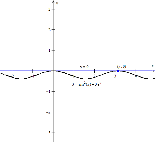
Find the equation of the tangent line for 3 = sin2(x) + 3ey at the point (p,0).
  • To construct a tangent line to a surface f we use x ×∇f(P) = P ×∇f(P), where x = (x,y) and P is the point of intersection between the plane and the surface.
  • Define f(x,y) = sin2(x) + 3ey − 3 and let P = (p,0). So ∇f(x,y) = ( 2sin(x)cos(x),3ey ).
  • Then x ×∇f(P) = P ×∇f(P) becomes (x,y) ×∇f(p,0) = (p,0) ×∇f(p,0) or (x,y) ×( 0,3 ) = (p,0) ×( 0,3 ).
Simplifying yields 3y = 0 or y = 0. To visualize the tangent line y = 0 to 3 = sin2(x) + 3ey we graph both on the same plane:
Find the equation of the tangent line for √2 = [3x/(y2)] at the point ( √2 , − √3 ).
  • To construct a tangent line to a surface f we use x ×∇f(P) = P ×∇f(P), where x = (x,y) and P is the point of intersection between the plane and the surface.
  • Define f(x,y) = [3x/(y2)] − √2 and let P = ( √2 , − √3 ). So ∇f(x,y) = ( [3/(y2)], − [6x/(y3)] ).
  • Then x ×∇f(P) = P ×∇f(P) becomes (x,y) ×∇f( √2 , − √3 ) = ( √2 , − √3 ) ×∇f( √2 , − √3 ) or (x,y) ×( 1,[(2√2 )/(√3 )] ) = ( √2 , − √3 ) ×( 1,[(2√2 )/(√3 )] ).
Simplifying yields x + [(2y√2 )/(√3 )] = √2 − 2√2 = − √2 or x√3 + 2y√2 = − √6 .
Find the equation of the tangent plane for − 51 = y2 − x2 − z at the point ( − 2,7,6).
  • To construct a tangent plane to a surface f we use x ×∇f(P) = P ×∇f(P), where x = (x,y,z) and P is the point of intersection between the plane and the surface.
  • Define f(x,y,z) = y2 − x2 − z + 51 and let P = ( − 2,7,6). So ∇f(x,y,z) = ( − 2x,2y, − 1 ).
  • Then x ×∇f(P) = P ×∇f(P) becomes (x,y,z) ×∇f( − 2,7,6) = ( − 2,7,6) ×∇f( − 2,7,6) or (x,y,z) ×( 4,14, − 1 ) = ( − 2,7,6) ×( 4,14, − 1 ).
Simplifying yields 4x + 14y − z = − 8 + 98 − 6 = 84 or 4x + 14y − z = 84.
Find the equation of the tangent plane for ln(3) − 1 = ln(2x + y) − z at the point (1,1, − 1).
  • To construct a tangent plane to a surface f we use x ×∇f(P) = P ×∇f(P), where x = (x,y,z) and P is the point of intersection between the plane and the surface.
  • Define f(x,y,z) = ln(2x + y) − z − ln(3) + 1 and let P = (1,1, − 1). So ∇f(x,y,z) = ( [2/(2x + y)],[1/(2x + y)], − 1 ). Then x ×∇f(P) = P ×∇f(P) becomes (x,y,z) ×∇f(1,1, − 1) = (1,1, − 1) ×∇f(1,1, − 1) or (x,y,z) ×( [2/3],[1/3], − 1 ) = (1,1, − 1) ×( [2/3],[1/3], − 1 ).
Simplifying yields [2/3]x + [1/3]y − z = [2/3] + [1/3] + 1 = 2 or 2x + y − 3z = 6.

*These practice questions are only helpful when you work on them offline on a piece of paper and then use the solution steps function to check your answer.

Answer

Tangent Plane

Lecture Slides are screen-captured images of important points in the lecture. Students can download and print out these lecture slide images to do practice problems as well as take notes while watching the lecture.

  • Intro 0:00
  • Tangent Plane 1:02
    • Tangent Plane Part 1
    • Tangent Plane Part 2
    • Tangent Plane Part 3
    • Tangent Plane Part 4
    • Definition 1: Tangent Plane to a Surface
    • Example 1: Find the Equation of the Plane Tangent to the Surface
    • Example 2: Find the Tangent Line to the Curve

Transcription: Tangent Plane

Hello and welcome back to educator.com and multi-variable calculus.0000

Today we are going to talk about a very, very important topic called the tangent plane and it is exactly what you think it is.0004

If you have a curve in space and you have some line, like in calculus when you did the derivative, you had the tangent to that curve, where this is the analog, the next level up.0010

If you have some surface in space, there is going to be some plane that is actually going to be tangent to it.0021

It is going to touch the surface at some point. We are going to devise a way using the gradient to come up with an equation for that tangent plane.0026

That tangent plane becomes very, very important throughout your studies. The whole idea of calculus is linearization.0035

When we linearize a curve, we take the tangent line. When we linearize a surface, we take the tangent plane, so it is very, very important.0042

Okay, let us just jump right on in. We are actually going to start off with an example in 2-dimensional space just to motivate it to get a clear picture of what is happening.0050

Then we will move on to three-dimensional space.0057

So, let us start with f(x,y), so a function of two variables, = x2 + y2.0064

This is just a parabaloid in 3-space.0074

Now, we will let our curve, we will let c(t) = cos(t) and sin(t).0079

As you remember, this is the parameterization for the unit circle in the plane, circle of radius 1.0090

Now, if we actually form f(c(t)), which we can because this is a mapping form R1 to R2, and this is a mapping from R2 to R1, we can go ahead and form the composite function f(c).0100

So, f(c) = f(c)... do it that way, because this is our functional notation and that is what we are used to seeing.0113

You know what, I am actually going to start avoid writing the t's, simply to make the notation a little more transparent and clear, not quite so busy.0121

But, of course we know... we aware of the functions so we are aware of the variables we are talking about, t and x and y.0131

But I hope it is okay if you just allow me to write f(c). Now if I put f(c), so wherever I have an x I put cos(t) so this is going to be cos2(t) + and wherever I have a y I put sin(t), so sin2(t).0140

As you know from your trig identities, cos2(t) + sin2(t), that is equal to 1.0155

So, now let us go ahead and examine the level curve. So, let us examine... and as you remember a level curve is the set of points for that function that when you put it into that function it equals a constant.0161

It is the set of points where they equal the same number over and over and over again.0177

So, let us examine the level curve f(x,y) = 1.0184

In other words, what we are saying is, so x2 + y2 = 1.0198

Now, this... so in 3-space this thing is the parabaloid that goes up, centered at the z axis.0205

When we actually set f(x,y) equal to some constant, what it is, it is actually some curve on there.0216

Then when you look at this from above, you are actually looking down on the x, y plane.0225

When you look down the z-axis, you are looking down on the x,y plane, and what you get is this curve in 2-space, the x,y plane.0231

Well this curve, for f(x,y) = 1, happens to be the unit circle. So, the level curve happens to be the same as the parameterization, in other words the curve itself, cos(t) sin(t) happens to lie right on the level surface for f(x,y) = 1. That is what is going on here.0242

So, recall... I am actually going to write everything out here... recall a level curve for f is the set of points x such that -- x is a vector here -- set of points x such that f(x) = k, a constant. That is it.0262

Just thought I would remind us of that. In this case k = 1. That is all that is happening here. k = 1.0293

So, again, you have the level curve and you have the parameterization, the curve itself, the curve and the function are actually 2 separate things, but as it turns out, this particular curve happens to correspond, happens to lie right on the level curve for the function f(x,y) = 1.0308

Alright. Now we can go ahead and start to do some Calculus.0329

So, the gradient of f -- well, it equals df/dx and df/dy, the gradient is a vector.0335

df/dx = 2x and df/dy = 2y.0351

The gradient of f evaluated at c, well 2x, x = cos(t), 2y, y = sin(t) because we are forming f(c).0360

That equals 2 × cos(t) and 2sin(t), so this is the gradient evaluated at c(t).0379

Now, let us do c'(t), well c'(t), that is just equal to -sin(t) and the derivative of cos is -- sorry the derivative of sin is cos(t), right?0391

So, this is the derivative of that, and this is the gradient, which is the derivative of the function and we ended up putting in the values of c(t) in there.0405

Now we have this thing, and now we have this thing. Well? We know that the d(f(c)), d(t), in other words the derivative of the composite function is equal to the gradient of f evaluated at c, dotted with c'(t).0418

Now, let me actually do this in a slightly different color. Now I am going to take this thing and this thing and I am going to form the dot product.0437

I am going to do this × this + this × this.0443

So, we end up getting this × this is -2sin(t)cos(t).0447

Then this is + this × this, 2sin(t)cos(t) -- -2sin(t)cos(t) + 2sin(t)cos(t), that equals 0.0458

So, what I have got here is the gradient of f at c dotted wtih c'(t) = 0.0471

Anytime you have 2 vectors, when you take the dot product and it equals 0, that means they are orthogonal.0480

That is the definition of orthogonality, or if you do not like the word orthogonal, perpendicular, it is just fine.0485

As it turns out, what you have here is that any time you have some function of 2 variables, again we are working with 2 variables here for this first example.0491

If you are going to form a composite function, in other words if the argument you put in to x and y, the values of x and y, happen to come from a parameterized curve, and if the curve happens to lie on the level curve, so if you have f(x,y) = some constant, f(c) = some constant,0502

As it turns out, the velocity vector of the curve and the gradient vector of the function are always going to be perpendicular to each other.0524

Pictorially, this looks like this. So this is the x,y plane, this is the unit circle, right?0532

This happens to be the level curve for x2 + y2 = 1.0543

So, x2 + y2 = 1, that is this. It also happens to be the curve that is parameterized by cos(t)sin(t).0549

The curve itself lies on this, the points that form the level curve of the function.0558

Now, the velocity vector, is this. c'(t), that is the velocity vector, so this is c', this vector right here.0565

The gradient vector is this, this is the gradient of f, they are perpendicular to each other. This will always be the case, this is not an accident.0574

Now, let us go ahead and generalize and move on to 3-space, and then we will go ahead and do a little discussion of 3-space, draw some pictures, try to make it as clear as possible, and then we will finish off with some examples.0585

So, again... well, let us just go ahead and move along here.0600

Now, let us let... should I go back to blue, it is ok, I will just leave it as blue -- you know what I think I will do this in black, excuse me.0603

Let us go back to black here. Alright, now we will let c be a mapping from R to R3, in other words a curve in 3-space.0616

A curve in 3-space... whoops, one of these days I will learn to write... we will let f be a mapping from R3 to R.0634

Okay, a function of 3 variables. Nice and simple, okay, so we can form f(c).0652

C maps from R to to R3, f maps from R3 to R, so we can take values from R3, put them into here so we can form f(c).0663

So, we can form, f(c), which is a mapping from R to R.0673

It is this R to this R. That is the composite function -- sorry to keep repeating myself, I just think it is important to keep doing that until it is completely natural.0685

We can differentiate this composite function, we can differentiate f(c).0700

So, we do d, f(c)dt, well we know what that is, that is equal to the gradient of f evaluated at c, dotted with c'(t).0712

Again, I am leaving off the t and things like that just to make the notation a little bit clearer.0730

Now let us consider the level surfaces of f. Now, consider the level surfaces of f.0735

In other words, the points in R3 where f(x,y,z) is equal to k, some constant -- let me make my k's a little better, I think these look like h's -- which is a constant.0750

This is also an important feature, and where the gradient of f(x,y,z), in other words at that point, well, the gradient everywhere does not equal 0.0780

So, when we say this... so, consider the level surfaces of f, when we had a function of 2 variables, that was a surface in 3-space, the level when that function = a constant, what we get is a level curve in 2-space.0794

Now what we are doing is we are moving onto a function of 3 variables. There we got level curves. Here, for a function of 3 variables, when f(x,y,z) is equal to some constant k, 14, what you get are a series of level surface.0812

You get surface in 3-space. So let us say x2 + y2 + z2 = 5, or x2 + y2 + z2 = 25.0828

These are spherical shells. So they are just places where the value of the function is constant and they are actually surfaces in 3-space, so we call them level surfaces.0839

In 2-space, we call them level curves. The general term is level surface.0848

This is actually really important. This gradient, not equal to 0, this basically says that the surface is smooth.0853

This is analogous to the derivative not being equal to 0, the derivative being defined.0862

Anywhere that the gradient is actually equal to 0, we can show that there are some problems there.0868

Here, where we said the gradient is not equal to 0, we just mean that it is a smooth curve, that is has no... it is not like it goes like this and then boom, there is some corner or something like that.0876

That is all this means when we say that the gradient is not equal to 0. It is just an extra feature that we take on here just to make sure that we are dealing with a surface that is well behaved.0884

Now, we say the curve c lies on the level surface if for all t, f(c(t)) is equal to k.0897

In other words, the points on the curve satisfy the equation for the level surface.0935

So, we had the function of 3 variables. We want to consider a particular level surface on f(x,y,z) = 15.0942

Well, because we form the composite function, if there was some curve that passes through R3, and if that curve happens to lie on the value, on the surface itself, in other words, the x, y, z values of the curve, such that when you put them into f(x,y,z) to form this composite function, f(c).0948

When those points satisfy the equation for the level surface. That is what we want to consider. We say that the curve lies on the level surface.0973

I will draw this out in a minute so you will actually see it.0985

In other words, the points on the curve satisfy the equation for the level surface.0988

What you are looking at is just this. Let me go ahead and draw a surface first, I will have something like this, and maybe like this, and maybe like that, and maybe like that.1018

So, here we have let us say the z-axis and I will go ahead and draw, this will be behind, of course I have that axis, and this axis.1033

This is the z, so this is the x, this is the z, and this is the y. That is basically just some surface in the x,y,z, plane... I am sorry in the x,y,z, space.1049

Now, here, if you have some curve itself, that happens to lie on the surface, well, since this is a level surface, the points (x,y,z) happen to satisfy f(x,y,z) equal a constant.1066

If the curve itself happens to lie on the surface, the points on the curve satisfy f(x,y,z) = that.1084

So f(c(t)) = the constant, that is all we are saying. That is all that is going on here.1092

Okay, now when we differentiate this, so when we differentiate f(c) = K, we get, well, on the left hand side, we get... remember? differentiating f(c), gradf(c) × c', gradf(c) · c' = 0.1099

Because, when we take the derivative of a constant, it is equal to 0.1138

So, c'(t) and gradient of f at c are perpendicular, just like we saw for... this is always going to be the case.1143

In other words, if I took that surface and I looked at it in such a way where I was just looking at the curve, I might have some curve like this... well c'(t) is going to be that vector.1164

As it turns out, so this is going to be c'(t), and this vector right here, this is going to be gradient of f at c.1176

This point right here, that is c(t), and this actually, this curve is actually on a surface.1187

All I have done is I have changed, taken the surface, so now I am looking at it like a cross-sectional view of the surface. Now I am just looking at the curve, that is all that is going on here.1194

Now, let me draw this in 3-dimensional perspective. So I have some surface, let us say something that looks like this, and I have this axis.1204

So it is very, very important. Again, we want to use geometry to help our intuition, but again this is really more about algebra.1217

Because again, when you are dealing with functions of more than 3 variables, 4, 5, 6, you can not rely on this.1227

We are just using this to help us understand what is happening physically, so that we can sort of put it together in our minds. That is all geometry is used for.1233

Essentially, this is some surface, and again we said that there is some curve that happens to lie on this level surface.1243

Well, if there is, that is going to be c'(t), and this is going to be the gradient of f at c.1250

Of course, this point right here, that is c(t) and this is perpendicular. That is all that is going on.1264

Now, I am going to draw one more picture and it is going to be the next one here, and then I will go ahead and actually write out some specific formal definitions.1277

A lot of this was just motivation. Now let us do one more picture, so, let me draw one more surface here. Something like that.1288

We have the z-axis, this comes down here, this is going to be the y-axis, and this is going to be the x-axis.1297

You know what, I will go ahead and label them. I mean at this point we should know which x's we are talking about.1308

So we have some point, this is going to be some point, now as it turns out, when you have a surface, there is more than 1 line that actually crosses that point.1313

You can have any kind of curve you want, that is the whole idea, you are not sort of stuck on one curve.1323

When you have this level surface in 3-space, there are a whole bunch of curves that pass over it, there is the curve this way, the curve this way, the curve this way.1330

If those curves that are parameterized at c(t) happen to lie on that surface, then the gradient vector and the velocity vector are always going to be perpendicular, so let me draw several curves that pass through this point.1338

So, you will have one curve that way, and another curve that way, and another curve that way. That is what is going on, as it turns out, the gradient vector is going to be perpendicular to every one of those curves.1356

This is actually very, very convenient. Now, let me call this point p, okay? Now let us write something down here. We will let p be a point on the level surface of the function f.1370

Now, let c be a curve passing through p, so some curve that happens to pass through p.1398

Well, then there is some value, let me write c(t) here, this is one of the... so c(t).1417

So let c(t) be a curve that happens to pass through t, so it is any one of these curves, an infinite number of them.1432

There is some value t0, such that the gradient of f evaluated at p, dotted with c'(t0) = 0.1439

So, we know that if a point on the curve happens to correspond, happens to actually lie on the level surface of the function, we know that the gradient vector × the velocity vector of the curve, c'(t), the dot product of those is equal to 0. We know it is perpendicular.1460

Okay, well, there are many such curves, as you can see. There are a whole bunch of curves that pass through that point.1481

Each one has its own velocity vector. So let us do another curve like that, there is another velocity vector, so I have 1, 2, 3, 4, and there is another velocity vector right there.1487

So, each one of those curves passes through that point, so there is an infinite number of them.1507

Each one has a velocity vector. Each one of those velocity vectors is perpendicular to the gradient, so what you have is this.1512

If you have some gradient vector like this, and if you have a curve passing this way, there is going to be this vector that is perpendicular.1520

Let us say you have a curve passing this way, this vector is perpendicular.1526

As it turns out, if I take all of these vectors all the way around, what I end up with is a plane, because all of these vectors are perpendicular, they all lie in the same plane.1531

Now we can go ahead and write out our definition.1544

I hope that made sense. So here we have our gradient vector, and then here we have all of these curves with all of their velocity vectors.1553

Well, since each one of those velocity vectors is perpendicular to the gradient vector, this is perpendicular, that is perpendicular, that is perpendicular.1561

If I actually move around and connect all of the vectors, since they are all perpendicular, they all lie in the same plane, all of the velocity vectors at that point p, they all lie in the same plane.1571

So what I have is the definition of a tangent plane to the surface at that point.1582

Now, let me go ahead and write down the definition.1590

You know what, let me write a couple of more things here just to make sure that it is specifically written down.1594

So, there are many curves on the level surface passing through p, and each has its own c'(t), 0.1601

All of these, c', all of these c'(0) form a plane.1638

So, we now make the following definition.1654

Okay... love definitions... here we go, now we finally get to the heart of the matter.1666

The tangent plane to a surface f(x) = k, notice I used the vector here instead of writing x,y,z.1675

Vector is just the short form instead of writing x, y, z, that is the component form.1693

So the tangent plane to a surface, f(x) = k at the point p is the plane passing through p -- I am going to write and -- and perpendicular to the gradient vector of f at p.1701

Now we remember... well, if we do not remember we will recall it here... the definition how we find the equation of a plane is we basically find... well, here is the definition of a plane.1744

It is x · n = p · n.1760

Well, if you have a plane, n is the normal, it is the vector that is perpendicular to that plane. Normal, remember normal and perpendicular?1767

So if we take x, which is just the variables x,y,z,q, whatever... and dot it with that, that is going to equal the point p dotted with that.1779

If you do not recall, go back to one of the previous lessons to where we motivated this particular way of finding the equation of a plane.1789

Now we have the tangent plane to a surface, to a level surface of f, or f(x) = k at the point p, it is the plane that passes through p and is perpendicular to the gradient vector.1798

Now n, our normal vector is the actual gradient vector, and it is based on what it is that we just discussed.1809

The fact that the gradient vector is going to be perpendicular to every single curve that happens to pass through that level surface.1816

All of the velocity vectors, they form a plane. That is what we call the tangent plane.1822

This is the general definition, here is what we are looking for.1828

x · the gradient of f at p = p · gradient of f at p.1833

This is the equation for a plane, for a tangent plane to the surface passing through the point p.1847

When we have our gradient vector, f at p, and when we have our point p, we go ahead and form this equation.1855

We multiply everything out, we take the dot product, we combine things, cancel things, whatever it is we need to do, and we are left with our equation for a plane.1862

Not let us go ahead and jump into some examples and hopefully it will make a lot more sense.1870

Let us see, alright... I will keep it in blue. So, this is example 1.1876

Okay, find the equation of the plane tangent to the surface x2 + y2 + z2 = 5.1884

Okay, at the point p, which is (1,2,1). Nice.1917

So we want to find the equation of the plane that is tangent to that surface at the point (1,2,1).1925

Now, we have our f, our function is x2 + y2 + z2.1934

Hopefully you will recognize this, this happens to be the equation of a sphere of radius sqrt(5) in 3-space. It is okay if you do not.1945

Remember, this is x2 + y2 + z2. That is a sphere. It is moving 1 dimension up from x2 + y2 = r2, where you have a circle in the x,y plane.1955

Let us go ahead and form the gradient, nice and easy. The gradient of f = well, the derivative with respect to x is 2x. The derivative with respect to y is 2y, the derivative with respect to z is 2z.1966

Nice and straight forward. Now when you evaluate that at p, in other words when you put (1,2,1) in for (x,y,z), we get the following.1980

This is going to equal, 2 × 1 is 2, and 2 × 2 is 4, and 2 × 1 is 2, so we get the vector (2,4,2).1988

Now we just form our equation. This thing right here. We take x... yeah, that is fine, so I will write it as x · the gradient of f at p = p · gradient of f at p.1998

This is just this. I am about to write the equation over and over again, it sort of gets me in the habit of thinking about it, remembering it, things like that.2019

Now that we actually have our vectors, now we do the component form. Whenever we do computations, we are working with components. Whenever we write out the theorems, the definitions, we keep it in form like this.2028

This is how you want to remember it, but you want to remember that vectors come as components.2038

Now, we will let x, let the variable x equal... let us just call it (x,y,z), that is not a problem... so I am going to need to go to the next page here.2045

We have what we just did, x, so which is (x,y,z) dotted with the gradient and the vector that we got was (2,4,2), that is equal to p, which was (1,2,1) dotted with (2,4,2).2062

Now we just do the dot product. This × this is 2x + 4y + 2z, make this a little more clear, = 1 × 2 is 2, 2 × 4 is 8, 1 × 2 is 2, that is equal to 12.2082

We get 2x + 4y + 2z = 12. There you go. This is the equation of the plane that passes through p and is tangent to the level surface of that function, at that point p.2101

Here is what it looks like. I am going to draw out a... yeah, let me go ahead and... so we said that x2 + y2 + z2 is equal to 5 is the sphere centered at the origin of radius sqrt(5).2118

So, it looks like this. I am going to draw it only in the first quadrant, and now I am going to go ahead and actually erase... yeah, let me make these a little bit clearer here so that you know that we are looking at a sphere.2138

So, this point... hopefully that is clear, so you have it in the first quadrant, and now the point (1,2,1) well this is the x-axis, this is the y-axis, and this is the z-axis, so 1 along the x-axis, 2 along the y and 1 along the z.2159

That is going to be some point right about there on the surface. What you want end up having is, of course, this plane that is touching that point and is tangent to it.2181

What you have is this... if I turn this around, what you would see is this curve, that part of the sphere, and you would have a tangent plane like that. That is what we found.2196

We found the equation for that plane, hitting, that touches the surface at that point, that is it. Nice and basic.2206

Let us go ahead and do another example here. We will finish off with this one. This is example 2.2215

This time we want to find the tangent line to the curve xy2 + x3 = 10 at the point (1,2).2227

So, notice. We said the tangent line at the curve. This whole, let me go back to black here for a second, this whole x · n = p · n, this is true in any number of dimensions. This is the general form of the equation.2264

Whether we are working in 3-space, 2-space, 15-space, that is the equation that we work.2284

Like we said before, when you have a curve, you have a tangent line. When you have a surface, you have a tangent plane.2290

Now let us move on to another dimension. When you have a surface in 4-space, well, you are going to have something that we call the hyper-plane, but we still use the same language for 3-dimensional space.2296

You are going to have a plane, you cannot draw it out, but that is what you have. This equation still works, even though we are talking about a tangent line and a curve, as opposed to a tangent plane and a surface.2309

It is the same equation. In other words, it is still going to be x · the gradient of f at p is equal to p · gradient of f at p.2320

That is what is wonderful about this. This equation is universal, and that is the whole idea. We want to generate it abstract so that it works in any number of dimensions, not just 1 or 2.2331

Okay, so let me go back to blue here. So, what we want is again, let me write it one more time. I know that it is a little redundant, but it is always good to write.2343

Gradient of f at p = p · gradient of f at p. Of course, these are that way.2354

We are going to let x = of course, (x,y), that is the component form. Well our f(x,y), or let us just say our f, let us leave off as many variables as we can, is xy2 + x3.2365

Let us go ahead and form the gradient. The gradient of f is equal to, well, it is equal to the first derivative of f, the second derivative of f, and that is going to equal y2 + 3x2.2383

That is the partial derivative of f with respect to x. We are holding y constant, so we just treat this like a constant. That is why it is y2 + 3x2.2400

Then, the second derivative, which is the derivative with respect to y, in this case, this one does not matter, we are holding x constant so that goes to 0.2409

Here it becomes 2xy. That is it.2417

Now, nice and systematic, the gradient of f evaluated at p, we go ahead and put the values of p, (1,2) into this.2422

So, wherever we see an x we put a 1, wherever we see a y we put a 2. That equals... 22 is 4 + 3, and then 2 × 1 × 2 is 4, so we should get (7,4).2432

I hope that you are checking my arithmetic. So, when we put it back into that, now that we actually have some vectors to work with, x is (x,y).2448

The gradient of f at p is (7,4). p itself is (1,2), and the gradient of f at p is (7,4).2463

There we go. Now we do the dot product, this is 7x + 4y, 1 × 7 is 7, 2 × 4 is 8, and if I am not mistaken, we get 7x + 4y = 15.2476

There you go. Finding, in this case, this is the equation of the line that is tangent to this curve at that point. That is it. That is all that is going on.2497

You are just using the idea that the gradient vector, the velocity vector are perpendicular. That is always going to be the case.2511

Thank you for joining us here at educator.com, in the next lesson we are actually going to do more examples using the concepts that we have been studying recently.2522

Partial derivatives, tangent planes, gradients, just to make sure that we have a good technical understanding and we develop some comfort before we actually move on to the next topic which is going to be directional derivatives.2531

So next time, further examples, take care, talk to you soon.2541

Educator®

Please sign in to participate in this lecture discussion.

Resetting Your Password?
OR

Start Learning Now

Our free lessons will get you started (Adobe Flash® required).
Get immediate access to our entire library.

Membership Overview

  • Available 24/7. Unlimited Access to Our Entire Library.
  • Search and jump to exactly what you want to learn.
  • *Ask questions and get answers from the community and our teachers!
  • Practice questions with step-by-step solutions.
  • Download lecture slides for taking notes.
  • Track your course viewing progress.
  • Accessible anytime, anywhere with our Android and iOS apps.