Raffi Hovasapian

Raffi Hovasapian

Points & Vectors

Slide Duration:

Table of Contents

Section 1: Vectors
Points & Vectors

28m 23s

Intro
0:00
Points and Vectors
1:02
A Point in a Plane
1:03
A Point in Space
3:14
Notation for a Space of a Given Space
6:34
Introduction to Vectors
9:51
Adding Vectors
14:51
Example 1
16:52
Properties of Vector Addition
18:24
Example 2
21:01
Two More Properties of Vector Addition
24:16
Multiplication of a Vector by a Constant
25:27
Scalar Product & Norm

30m 25s

Intro
0:00
Scalar Product and Norm
1:05
Introduction to Scalar Product
1:06
Example 1
3:21
Properties of Scalar Product
6:14
Definition: Orthogonal
11:41
Example 2: Orthogonal
14:19
Definition: Norm of a Vector
15:30
Example 3
19:37
Distance Between Two Vectors
22:05
Example 4
27:19
More on Vectors & Norms

38m 18s

Intro
0:00
More on Vectors and Norms
0:38
Open Disc
0:39
Close Disc
3:14
Open Ball, Closed Ball, and the Sphere
5:22
Property and Definition of Unit Vector
7:16
Example 1
14:04
Three Special Unit Vectors
17:24
General Pythagorean Theorem
19:44
Projection
23:00
Example 2
28:35
Example 3
35:54
Inequalities & Parametric Lines

33m 19s

Intro
0:00
Inequalities and Parametric Lines
0:30
Starting Example
0:31
Theorem 1
5:10
Theorem 2
7:22
Definition 1: Parametric Equation of a Straight Line
10:16
Definition 2
17:38
Example 1
21:19
Example 2
25:20
Planes

29m 59s

Intro
0:00
Planes
0:18
Definition 1
0:19
Example 1
7:04
Example 2
12:45
General Definitions and Properties: 2 Vectors are Said to Be Paralleled If
14:50
Example 3
16:44
Example 4
20:17
More on Planes

34m 18s

Intro
0:00
More on Planes
0:25
Example 1
0:26
Distance From Some Point in Space to a Given Plane: Derivation
10:12
Final Formula for Distance
21:20
Example 2
23:09
Example 3: Part 1
26:56
Example 3: Part 2
31:46
Section 2: Differentiation of Vectors
Maps, Curves & Parameterizations

29m 48s

Intro
0:00
Maps, Curves and Parameterizations
1:10
Recall
1:11
Looking at y = x2 or f(x) = x2
2:23
Departure Space & Arrival Space
7:01
Looking at a 'Function' from ℝ to ℝ2
10:36
Example 1
14:50
Definition 1: Parameterized Curve
17:33
Example 2
21:56
Example 3
25:16
Differentiation of Vectors

39m 40s

Intro
0:00
Differentiation of Vectors
0:18
Example 1
0:19
Definition 1: Velocity of a Curve
1:45
Line Tangent to a Curve
6:10
Example 2
7:40
Definition 2: Speed of a Curve
12:18
Example 3
13:53
Definition 3: Acceleration Vector
16:37
Two Definitions for the Scalar Part of Acceleration
17:22
Rules for Differentiating Vectors: 1
19:52
Rules for Differentiating Vectors: 2
21:28
Rules for Differentiating Vectors: 3
22:03
Rules for Differentiating Vectors: 4
24:14
Example 4
26:57
Section 3: Functions of Several Variables
Functions of Several Variable

29m 31s

Intro
0:00
Length of a Curve in Space
0:25
Definition 1: Length of a Curve in Space
0:26
Extended Form
2:06
Example 1
3:40
Example 2
6:28
Functions of Several Variable
8:55
Functions of Several Variable
8:56
General Examples
11:11
Graph by Plotting
13:00
Example 1
16:31
Definition 1
18:33
Example 2
22:15
Equipotential Surfaces
25:27
Isothermal Surfaces
27:30
Partial Derivatives

23m 31s

Intro
0:00
Partial Derivatives
0:19
Example 1
0:20
Example 2
5:30
Example 3
7:48
Example 4
9:19
Definition 1
12:19
Example 5
14:24
Example 6
16:14
Notation and Properties for Gradient
20:26
Higher and Mixed Partial Derivatives

30m 48s

Intro
0:00
Higher and Mixed Partial Derivatives
0:45
Definition 1: Open Set
0:46
Notation: Partial Derivatives
5:39
Example 1
12:00
Theorem 1
14:25
Now Consider a Function of Three Variables
16:50
Example 2
20:09
Caution
23:16
Example 3
25:42
Section 4: Chain Rule and The Gradient
The Chain Rule

28m 3s

Intro
0:00
The Chain Rule
0:45
Conceptual Example
0:46
Example 1
5:10
The Chain Rule
10:11
Example 2: Part 1
19:06
Example 2: Part 2 - Solving Directly
25:26
Tangent Plane

42m 25s

Intro
0:00
Tangent Plane
1:02
Tangent Plane Part 1
1:03
Tangent Plane Part 2
10:00
Tangent Plane Part 3
18:18
Tangent Plane Part 4
21:18
Definition 1: Tangent Plane to a Surface
27:46
Example 1: Find the Equation of the Plane Tangent to the Surface
31:18
Example 2: Find the Tangent Line to the Curve
36:54
Further Examples with Gradients & Tangents

47m 11s

Intro
0:00
Example 1: Parametric Equation for the Line Tangent to the Curve of Two Intersecting Surfaces
0:41
Part 1: Question
0:42
Part 2: When Two Surfaces in ℝ3 Intersect
4:31
Part 3: Diagrams
7:36
Part 4: Solution
12:10
Part 5: Diagram of Final Answer
23:52
Example 2: Gradients & Composite Functions
26:42
Part 1: Question
26:43
Part 2: Solution
29:21
Example 3: Cos of the Angle Between the Surfaces
39:20
Part 1: Question
39:21
Part 2: Definition of Angle Between Two Surfaces
41:04
Part 3: Solution
42:39
Directional Derivative

41m 22s

Intro
0:00
Directional Derivative
0:10
Rate of Change & Direction Overview
0:11
Rate of Change : Function of Two Variables
4:32
Directional Derivative
10:13
Example 1
18:26
Examining Gradient of f(p) ∙ A When A is a Unit Vector
25:30
Directional Derivative of f(p)
31:03
Norm of the Gradient f(p)
33:23
Example 2
34:53
A Unified View of Derivatives for Mappings

39m 41s

Intro
0:00
A Unified View of Derivatives for Mappings
1:29
Derivatives for Mappings
1:30
Example 1
5:46
Example 2
8:25
Example 3
12:08
Example 4
14:35
Derivative for Mappings of Composite Function
17:47
Example 5
22:15
Example 6
28:42
Section 5: Maxima and Minima
Maxima & Minima

36m 41s

Intro
0:00
Maxima and Minima
0:35
Definition 1: Critical Point
0:36
Example 1: Find the Critical Values
2:48
Definition 2: Local Max & Local Min
10:03
Theorem 1
14:10
Example 2: Local Max, Min, and Extreme
18:28
Definition 3: Boundary Point
27:00
Definition 4: Closed Set
29:50
Definition 5: Bounded Set
31:32
Theorem 2
33:34
Further Examples with Extrema

32m 48s

Intro
0:00
Further Example with Extrema
1:02
Example 1: Max and Min Values of f on the Square
1:03
Example 2: Find the Extreme for f(x,y) = x² + 2y² - x
10:44
Example 3: Max and Min Value of f(x,y) = (x²+ y²)⁻¹ in the Region (x -2)²+ y² ≤ 1
17:20
Lagrange Multipliers

32m 32s

Intro
0:00
Lagrange Multipliers
1:13
Theorem 1
1:14
Method
6:35
Example 1: Find the Largest and Smallest Values that f Achieves Subject to g
9:14
Example 2: Find the Max & Min Values of f(x,y)= 3x + 4y on the Circle x² + y² = 1
22:18
More Lagrange Multiplier Examples

27m 42s

Intro
0:00
Example 1: Find the Point on the Surface z² -xy = 1 Closet to the Origin
0:54
Part 1
0:55
Part 2
7:37
Part 3
10:44
Example 2: Find the Max & Min of f(x,y) = x² + 2y - x on the Closed Disc of Radius 1 Centered at the Origin
16:05
Part 1
16:06
Part 2
19:33
Part 3
23:17
Lagrange Multipliers, Continued

31m 47s

Intro
0:00
Lagrange Multipliers
0:42
First Example of Lesson 20
0:44
Let's Look at This Geometrically
3:12
Example 1: Lagrange Multiplier Problem with 2 Constraints
8:42
Part 1: Question
8:43
Part 2: What We Have to Solve
15:13
Part 3: Case 1
20:49
Part 4: Case 2
22:59
Part 5: Final Solution
25:45
Section 6: Line Integrals and Potential Functions
Line Integrals

36m 8s

Intro
0:00
Line Integrals
0:18
Introduction to Line Integrals
0:19
Definition 1: Vector Field
3:57
Example 1
5:46
Example 2: Gradient Operator & Vector Field
8:06
Example 3
12:19
Vector Field, Curve in Space & Line Integrals
14:07
Definition 2: F(C(t)) ∙ C'(t) is a Function of t
17:45
Example 4
18:10
Definition 3: Line Integrals
20:21
Example 5
25:00
Example 6
30:33
More on Line Integrals

28m 4s

Intro
0:00
More on Line Integrals
0:10
Line Integrals Notation
0:11
Curve Given in Non-parameterized Way: In General
4:34
Curve Given in Non-parameterized Way: For the Circle of Radius r
6:07
Curve Given in Non-parameterized Way: For a Straight Line Segment Between P & Q
6:32
The Integral is Independent of the Parameterization Chosen
7:17
Example 1: Find the Integral on the Ellipse Centered at the Origin
9:18
Example 2: Find the Integral of the Vector Field
16:26
Discussion of Result and Vector Field for Example 2
23:52
Graphical Example
26:03
Line Integrals, Part 3

29m 30s

Intro
0:00
Line Integrals
0:12
Piecewise Continuous Path
0:13
Closed Path
1:47
Example 1: Find the Integral
3:50
The Reverse Path
14:14
Theorem 1
16:18
Parameterization for the Reverse Path
17:24
Example 2
18:50
Line Integrals of Functions on ℝn
21:36
Example 3
24:20
Potential Functions

40m 19s

Intro
0:00
Potential Functions
0:08
Definition 1: Potential Functions
0:09
Definition 2: An Open Set S is Called Connected if…
5:52
Theorem 1
8:19
Existence of a Potential Function
11:04
Theorem 2
18:06
Example 1
22:18
Contrapositive and Positive Form of the Theorem
28:02
The Converse is Not Generally True
30:59
Our Theorem
32:55
Compare the n-th Term Test for Divergence of an Infinite Series
36:00
So for Our Theorem
38:16
Potential Functions, Continued

31m 45s

Intro
0:00
Potential Functions
0:52
Theorem 1
0:53
Example 1
4:00
Theorem in 3-Space
14:07
Example 2
17:53
Example 3
24:07
Potential Functions, Conclusion & Summary

28m 22s

Intro
0:00
Potential Functions
0:16
Theorem 1
0:17
In Other Words
3:25
Corollary
5:22
Example 1
7:45
Theorem 2
11:34
Summary on Potential Functions 1
15:32
Summary on Potential Functions 2
17:26
Summary on Potential Functions 3
18:43
Case 1
19:24
Case 2
20:48
Case 3
21:35
Example 2
23:59
Section 7: Double Integrals
Double Integrals

29m 46s

Intro
0:00
Double Integrals
0:52
Introduction to Double Integrals
0:53
Function with Two Variables
3:39
Example 1: Find the Integral of xy³ over the Region x ϵ[1,2] & y ϵ[4,6]
9:42
Example 2: f(x,y) = x²y & R be the Region Such That x ϵ[2,3] & x² ≤ y ≤ x³
15:07
Example 3: f(x,y) = 4xy over the Region Bounded by y= 0, y= x, and y= -x+3
19:20
Polar Coordinates

36m 17s

Intro
0:00
Polar Coordinates
0:50
Polar Coordinates
0:51
Example 1: Let (x,y) = (6,√6), Convert to Polar Coordinates
3:24
Example 2: Express the Circle (x-2)² + y² = 4 in Polar Form.
5:46
Graphing Function in Polar Form.
10:02
Converting a Region in the xy-plane to Polar Coordinates
14:14
Example 3: Find the Integral over the Region Bounded by the Semicircle
20:06
Example 4: Find the Integral over the Region
27:57
Example 5: Find the Integral of f(x,y) = x² over the Region Contained by r= 1 - cosθ
32:55
Green's Theorem

38m 1s

Intro
0:00
Green's Theorem
0:38
Introduction to Green's Theorem and Notations
0:39
Green's Theorem
3:17
Example 1: Find the Integral of the Vector Field around the Ellipse
8:30
Verifying Green's Theorem with Example 1
15:35
A More General Version of Green's Theorem
20:03
Example 2
22:59
Example 3
26:30
Example 4
32:05
Divergence & Curl of a Vector Field

37m 16s

Intro
0:00
Divergence & Curl of a Vector Field
0:18
Definitions: Divergence(F) & Curl(F)
0:19
Example 1: Evaluate Divergence(F) and Curl(F)
3:43
Properties of Divergence
9:24
Properties of Curl
12:24
Two Versions of Green's Theorem: Circulation - Curl
17:46
Two Versions of Green's Theorem: Flux Divergence
19:09
Circulation-Curl Part 1
20:08
Circulation-Curl Part 2
28:29
Example 2
32:06
Divergence & Curl, Continued

33m 7s

Intro
0:00
Divergence & Curl, Continued
0:24
Divergence Part 1
0:25
Divergence Part 2: Right Normal Vector and Left Normal Vector
5:28
Divergence Part 3
9:09
Divergence Part 4
13:51
Divergence Part 5
19:19
Example 1
23:40
Final Comments on Divergence & Curl

16m 49s

Intro
0:00
Final Comments on Divergence and Curl
0:37
Several Symbolic Representations for Green's Theorem
0:38
Circulation-Curl
9:44
Flux Divergence
11:02
Closing Comments on Divergence and Curl
15:04
Section 8: Triple Integrals
Triple Integrals

27m 24s

Intro
0:00
Triple Integrals
0:21
Example 1
2:01
Example 2
9:42
Example 3
15:25
Example 4
20:54
Cylindrical & Spherical Coordinates

35m 33s

Intro
0:00
Cylindrical and Spherical Coordinates
0:42
Cylindrical Coordinates
0:43
When Integrating Over a Region in 3-space, Upon Transformation the Triple Integral Becomes..
4:29
Example 1
6:27
The Cartesian Integral
15:00
Introduction to Spherical Coordinates
19:44
Reason It's Called Spherical Coordinates
22:49
Spherical Transformation
26:12
Example 2
29:23
Section 9: Surface Integrals and Stokes' Theorem
Parameterizing Surfaces & Cross Product

41m 29s

Intro
0:00
Parameterizing Surfaces
0:40
Describing a Line or a Curve Parametrically
0:41
Describing a Line or a Curve Parametrically: Example
1:52
Describing a Surface Parametrically
2:58
Describing a Surface Parametrically: Example
5:30
Recall: Parameterizations are not Unique
7:18
Example 1: Sphere of Radius R
8:22
Example 2: Another P for the Sphere of Radius R
10:52
This is True in General
13:35
Example 3: Paraboloid
15:05
Example 4: A Surface of Revolution around z-axis
18:10
Cross Product
23:15
Defining Cross Product
23:16
Example 5: Part 1
28:04
Example 5: Part 2 - Right Hand Rule
32:31
Example 6
37:20
Tangent Plane & Normal Vector to a Surface

37m 6s

Intro
0:00
Tangent Plane and Normal Vector to a Surface
0:35
Tangent Plane and Normal Vector to a Surface Part 1
0:36
Tangent Plane and Normal Vector to a Surface Part 2
5:22
Tangent Plane and Normal Vector to a Surface Part 3
13:42
Example 1: Question & Solution
17:59
Example 1: Illustrative Explanation of the Solution
28:37
Example 2: Question & Solution
30:55
Example 2: Illustrative Explanation of the Solution
35:10
Surface Area

32m 48s

Intro
0:00
Surface Area
0:27
Introduction to Surface Area
0:28
Given a Surface in 3-space and a Parameterization P
3:31
Defining Surface Area
7:46
Curve Length
10:52
Example 1: Find the Are of a Sphere of Radius R
15:03
Example 2: Find the Area of the Paraboloid z= x² + y² for 0 ≤ z ≤ 5
19:10
Example 2: Writing the Answer in Polar Coordinates
28:07
Surface Integrals

46m 52s

Intro
0:00
Surface Integrals
0:25
Introduction to Surface Integrals
0:26
General Integral for Surface Are of Any Parameterization
3:03
Integral of a Function Over a Surface
4:47
Example 1
9:53
Integral of a Vector Field Over a Surface
17:20
Example 2
22:15
Side Note: Be Very Careful
28:58
Example 3
30:42
Summary
43:57
Divergence & Curl in 3-Space

23m 40s

Intro
0:00
Divergence and Curl in 3-Space
0:26
Introduction to Divergence and Curl in 3-Space
0:27
Define: Divergence of F
2:50
Define: Curl of F
4:12
The Del Operator
6:25
Symbolically: Div(F)
9:03
Symbolically: Curl(F)
10:50
Example 1
14:07
Example 2
18:01
Divergence Theorem in 3-Space

34m 12s

Intro
0:00
Divergence Theorem in 3-Space
0:36
Green's Flux-Divergence
0:37
Divergence Theorem in 3-Space
3:34
Note: Closed Surface
6:43
Figure: Paraboloid
8:44
Example 1
12:13
Example 2
18:50
Recap for Surfaces: Introduction
27:50
Recap for Surfaces: Surface Area
29:16
Recap for Surfaces: Surface Integral of a Function
29:50
Recap for Surfaces: Surface Integral of a Vector Field
30:39
Recap for Surfaces: Divergence Theorem
32:32
Stokes' Theorem, Part 1

22m 1s

Intro
0:00
Stokes' Theorem
0:25
Recall Circulation-Curl Version of Green's Theorem
0:26
Constructing a Surface in 3-Space
2:26
Stokes' Theorem
5:34
Note on Curve and Vector Field in 3-Space
9:50
Example 1: Find the Circulation of F around the Curve
12:40
Part 1: Question
12:48
Part 2: Drawing the Figure
13:56
Part 3: Solution
16:08
Stokes' Theorem, Part 2

20m 32s

Intro
0:00
Example 1: Calculate the Boundary of the Surface and the Circulation of F around this Boundary
0:30
Part 1: Question
0:31
Part 2: Drawing the Figure
2:02
Part 3: Solution
5:24
Example 2: Calculate the Boundary of the Surface and the Circulation of F around this Boundary
13:11
Part 1: Question
13:12
Part 2: Solution
13:56
Loading...
This is a quick preview of the lesson. For full access, please Log In or Sign up.
For more information, please see full course syllabus of Multivariable Calculus
Bookmark & Share Embed

Share this knowledge with your friends!

Copy & Paste this embed code into your website’s HTML

Please ensure that your website editor is in text mode when you paste the code.
(In Wordpress, the mode button is on the top right corner.)
  ×
  • - Allow users to view the embedded video in full-size.
  • Discussion

  • Answer Engine

  • Practice Questions

  • Download Lecture Slides

  • Table of Contents

  • Transcription

  • Related Books

Lecture Comments (17)

1 answer

Last reply by: Professor Hovasapian
Mon Feb 1, 2016 5:19 AM

Post by Gowrish Vaka on January 31, 2016

Dr. Hovasapian,
I was wondering if it is reasonable to learn multivariable Calculus as a high school senior. I have taken AP Calculus BC and earned a 5 on both portions: AB and BC. Is it wise for me to head to multivariable Calculus, or would it be better for me to learn College Calc I and Calc II before?

Thank You

1 answer

Last reply by: Professor Hovasapian
Mon Dec 21, 2015 7:34 PM

Post by Mitchell Mayberry on December 21, 2015

Dr. Hovasapian,

I was just wondering how closely these lectures follow a normal college Calculus 3 agenda? Any information would be greatly appreciated.
 

0 answers

Post by Professor Hovasapian on September 10, 2013

Hi Yaqub,

I hope you're well.

Complex numbers, when represented in the 2-dimensional plane ARE vectors, because there are 2 components -- the x and the y. So a Complex number IS a 2-vector.

If the question is " can there be vectors with complex entries?", then also YES, absolutely. For example:

[2+3i, 5-i, 4-7i]

This is a 1X3 vector whose entries are complex.

If I take the complex number 3+4i, it IS a vector [3,4]

I hope that helps. Please let me know if I have misunderstood your question.

Best wishes.

Raffi

0 answers

Post by yaqub ali on September 10, 2013

can vectors exist in complex planes?

1 answer

Last reply by: Professor Hovasapian
Sun May 12, 2013 5:30 AM

Post by Lauran Bahr on May 10, 2013

Praise the lord you have made me see how I can actually learn again like I did in high school. Can we all keep our shirts on please? And yes I think you are good at teaching as well.

1 answer

Last reply by: Professor Hovasapian
Mon Jan 28, 2013 2:39 AM

Post by Josh Winfield on January 27, 2013

I am responding very well to your teaching approach. Thank you

0 answers

Post by Senghuot Lim on July 9, 2012

this guys is really good at teaching :)

5 answers

Last reply by: Professor Hovasapian
Fri Jul 27, 2012 6:34 PM

Post by Jonathan Bello on July 3, 2012

I wish this course was available last semester (spring '12) I would of passed this course. Now I will have to wait until next spring.

Points & Vectors

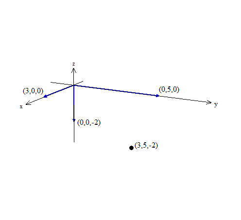
Graph the point (3,5, − 2) on R3.
  • Each number corresponds to an axis on three space, so that (3,5, − 2) has x = 3, y = 5 and z = − 2.
Graphing on the xyz - plane yields:
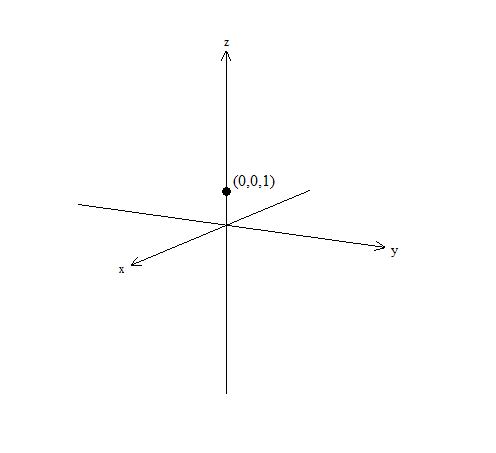
Graph the point (0,0,1) on R3.
  • Each number corresponds to an axis on three space, so that (0,0, − 1) has x = 0, y = 0 and z = − 1.
Graphing on the xyz - plane yields:
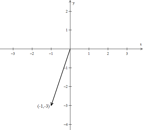
Graph the vector a = ( − 1, − 3) on R2.
  • Each number corresponds to an axis on two space, so that ( − 1, − 3) has x = − 1, y = − 3.
  • Note that since this is a vector, our endpoints are (0,0) and ( − 1, − 3).
Graphing on the xy - plane yields: (don't forget the arrow)
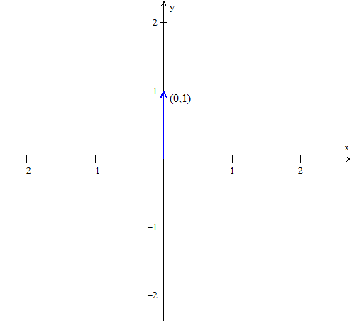
Graph the vector j = (0,1) on R2.
  • Each number corresponds to an axis on two space, so that (0,1) has x = 0, y = 1.
  • Note that since this is a vector, our endpoints are (0,0) and (0,1).
Graphing on the xy - plane yields: (don't forget the arrow)
For the following problems, let a = ( − 2,5, − 4), b = (6,1, − 1).
Find c = a + b
  • Substitute: c = a + b = ( − 2,5, − 4) + (6,1, − 1)
  • Add correspoinding axis: ( − 2,5, − 4) + (6,1, − 1) = ( − 2 + 6,5 + 1, − 4 + ( − 1))
Solution: c = (4,6, − 5).
Find d = b − a
  • Substitute: d = b − a = b + ( − a) = (6,1, − 1) + (2, − 5,4)
  • Add correspoinding axis: (6,1, − 1) + (2, − 5,4) = (6 + 2,1 + ( − 5), − 1 + 4)
Solution: c = (8, − 4,3).
For the following problems, let a = ( − 2,5, − 4), b = (6,1, − 1).
Find [1/2]a
  • Substitute: [1/2]a = [1/2]( − 2,5, − 4)
  • Multiply each coordinate: [1/2]( − 2,5, − 4) = ( [1/2] ×− 2,[1/2] ×5,[1/2] ×− 4 )
Solution: ( − 1,[5/2], − 2 )
Find − [3/2]b
  • Substitute: − [3/2]b = [3/2](6,1, − 1)
  • Multiply each coordinate: − [3/2](6,1, − 1) = ( − [3/2] ×6, − [3/2] ×1, − [3/2] ×− 1 )
Solution: ( − 9, − [3/2],[3/2] )
Find √2 a + 2√2 b
  • Note that √2 a + 2√2 b = √2 (a + 2b)
  • a + 2b = ( − 2,5, − 4) + (2 ×6,2 ×1,2 ×− 1) = ( − 2,5, − 4) + (12,2, − 2) = (10,7, − 6)
Solution: √2 (10,7, − 6) = (10√2 ,7√2 , − 6√2 )
Let a = (a1,a2,a3,a4), b = ( − a1,a2, − a3,a4) with a1,a2,a3,a4 being nonzero.
i) Find esa + b.
  • Substitute: a + b = (a1,a2,a3,a4) + ( − a1,a2, − a3,a4).
Add corresponding axis: (a1,a2,a3,a4) + ( − a1,a2, − a3,a4) = (a1 + ( − a1),a2 + a2,a3 + ( − a3),a4 + ( − a4)) = (0,2a2,0,2a4) = 2(0,a2,0,a4)
Let a = (a1,a2,a3,a4), b = ( − a1,a2, − a3,a4) with a1,a2,a3,a4 being nonzero.
ii) Is a + b = 0? Explain.
Recall that 0 = (0, …,0) for n dimensions, in other words, every entry is a zero. Our answer has two nonzero entries on the second and fourth coordinate. Hence a + b ≠ 0.

*These practice questions are only helpful when you work on them offline on a piece of paper and then use the solution steps function to check your answer.

Answer

Points & Vectors

Lecture Slides are screen-captured images of important points in the lecture. Students can download and print out these lecture slide images to do practice problems as well as take notes while watching the lecture.

  • Intro 0:00
  • Points and Vectors 1:02
    • A Point in a Plane
    • A Point in Space
    • Notation for a Space of a Given Space
    • Introduction to Vectors
    • Adding Vectors
    • Example 1
    • Properties of Vector Addition
    • Example 2
    • Two More Properties of Vector Addition
    • Multiplication of a Vector by a Constant

Transcription: Points & Vectors

Welcome to educator.com.0000

Welcome to the first lesson of multivariable calculus at educator.com.0006

Multi variable calculus is an extraordinary branch of mathematics.0010

Those of you who are coming to this course, you have already come from a course in regular calculus.0013

What we are going to do is, we are going to take the power of calculus, and we are going to move from one dimension.0016

We are just going to move up, to two dimensions, to three dimensions, and as it turns out, any number of dimensions.0023

That is what makes all the things that we are going to learn really, really exciting.0028

We are not limited to two and three dimensions, in general.0032

We are going to be doing most of our work in two and three dimensions, because we want to visualize things.0036

We are used to playing in space and things like that, but the results are valid for any number of dimensions.0040

So, let us jump right in and see what we can do. Welcome again.0047

We are going to start off with just some normal basics.0051

We are going to talk about points and vectors just to get ourselves going.0053

A lot of the stuff that you may have seen before, if you have not seen it before, it is reasonably straightforward.0056

Let us start off by just defining a point in space.0063

A point in space, can be identified... Actually, I am sorry, let us start with a point on a plane, not in space.0070

We will work ourselves into 3 space in just a minute.0082

A point on a plane can be identified with two numbers.0086

One number for the x-coordinate, and one number for the y-coordinate.0106

This is nothing that you have not been doing for years and years and years.0120

Just the normal Cartesian coordinate plane.0124

You have an X axis, and a Y axis, and when you choose a point in that plane you need 2 numbers to define where it is in that plane.0128

Let me just go ahead and finish writing off the y-coordinate.0134

So, a quick picture, you are going to have something like this.0137

This is the Cartesian coordinate plane and let us take a number like that.0140

So, this point might be (6,2).0146

In other words you are 6 in the x direction, this is the X axis only, the X axis is horizontal, Y axis is vertical, and 2 units in the Y direction.0147

That gives us a point in space.0157

Now, because we need two numbers to identify that point, we call that a two-dimensional space.0165

So, whenever you hear the word dimension, do not freak out, it is just a fancy word for number.0170

When we talk about a 17 dimensional space, it just means that in order to identify a space, or a point in that space, we need 17 numbers.0174

That is all it is, dimensions, numbers, they are synonymous.0181

Okay, so now let us actually talk about a point in space, the space that we think of as the space that we live in, the space that we know, 3 space.0188

So a point in 3 space, actually let us not identify it as 3 space yet, let us go nice and slow.0198

A point in space can, can be identified with 3 numbers.0210

Again, one for X, one for Y, and one for z, we generally do x-coordinate, y-coordinate, z-coordinate.0225

Let us go ahead and draw what this looks like.0239

This is going to be a standard coordinate system called the right-hand coordinate system for visualizing points in three-dimensional space.0243

What we have is something like this, slightly different.0249

This right here, this is actually the z axis, and this one that is slanted, this is actually going back and coming forward.0256

So, this z-axis and this Y-axis are actually the plane of the paper.0268

This right here is actually the X axis so, what we have done is we have taken the XY, we have flipped it down, and we have added a z-axis to it.0276

If you have some point like, I do not know, let us put a point over here, and let us call this point (3,3,2).0286

We have three numbers identifying that point.0296

That means that we have moved three units in the X direction, we have moved three units along the Y direction, and we have moved two units along the Z axis.0298

That is it, three-dimensional space, because we need three numbers to represent that point.0338

Now, analogously we can talk about any number of dimensions.0346

We can talk about five space, six space, seven space.0348

It just means we need 5, 6, 7, you know, numbers to identify a point in that space.0353

The behavior is exactly the same, even if we cannot visualize it.0360

In other words we are kind of limited to two dimensions and three dimensional representations theoretically,0365

But algebraically, we can just do, for example, if we have a space which is (4,7,6,5,9), this is a five dimensional space, this is a point in a five dimensional space.0370

We cannot visualize it, and we cannot draw it, but we can work with it algebraically.0384

Let us go ahead and talk about a notation briefly, a notation for a space of a given dimension.0392

This is a notation that we will use reasonably regularly.0408

We will start to use it more often when we talk about functions from say a two-dimensional space, to a one-dimensional space.0411

Taking a number that has, you know, two coordinates, and mapping it and doing something to those numbers, and coming up with an answer that ends up in a different space.0420

This notation that I am going to introduce, you will see it more later on, but I do want to introduce it right now.0432

So, R is the symbol for the real number system.0436

You will have R represents 1 space, and so when we say the space R, we are talking about one dimensional space.0450

In other words, a line.0459

Basically, you need just one number.0460

The reason we use R is because, you notice 2 space is 2 numbers, 3 spaces is 3 numbers, 5 spaces has 5 numbers,0463

Well you are taking these numbers, the 6, the 2, the 3, the 3,0470

You are taking them from the set of real numbers so R2, when we put a little two on top, that is two space.0474

It is saying that we are taking, well, this two tells us that we need two numbers, one from the real number system, another one from the real number system to identify that.0484

So R2 is 2 space, it is the Cartesian coordinate plane.0496

Oops, we are starting to get these crazy lines again.0499

Let us see if we can write a little bit slower to avoid some of that.0502

The real number system, actually, let me go ahead and move to the next page here.0506

So, R is 1 space, R2 is 2 space, and R3 is 3 space.0511

When we talk about the space that we live in, we are actually talking about R3.0532

In other words, three numbers from the real number system to identify a point in space,0536

We will be using that more when we talk about functions again.0540

OK, these points in space are actually individual objects.0544

You can think of them just like numbers.0550

For example, if I said I have the number 14 and the number 17,0552

These are individual mathematical objects, these points in space are also just single individual mathematical objects.0555

The difference is we need more than one number to actually describe them.0563

These numbers are the coordinates.0567

As you will see in a minute, these points in space which we are actually going to start to call vectors in a minute, they are individual objects, and we treat them like individual objects that you can treat just like numbers.0572

It is just that they happen to be made up of more than one thing.0582

It will make more sense as we start to do the problems.0587

OK, so now let us go ahead and talk about vectors.0595

We often call points in space, vectors, and in fact, that is probably going to be the primary term that I use.0601

It is just so ubiquitous, so common in mathematics to speak about a point in space as a vector.0613

We will go ahead and get into the geometry a little bit, but just know that it is just another term for a point in space, that is all it is.0621

So (1,-7) a point in two space is called a 2 vector, and exactly what you might think,0629

The point (3,-4,6) is a 3 vector, that is it.0644

The reason we call it a vector is, again, some of you people might have seen vectors in physics or another math course, perhaps some of your calculus courses actually talked about vectors, I do not know.0653

Occasionally they do.0667

We call them vectors because you can actually think of a point in two ways.0668

You can think that it is just a point in space, or you can think of it as an arrow from the origin to that point in space.0672

Let us go ahead and draw it out.0681

The geometry would be something like this.0683

So, if I had some random point, so this is the x-y plane, and if I had the point (6,2), that is a point.0686

You know 6 along the X axis, 2 along the y-axis,0690

But it also represents an arrow, an actual direction from a point of origin in this case, the origin, in that direction.0700

This is called a vector and it is a directed line segment.0708

It is not just a point in space, it actually gives us a direction and that is why we call it a vector.0712

So there are two ways of looking at it.0719

In general, we will be using these arrows in 2 and 3 dimensions, mostly we will be working in two-dimensions when we do the examples,0725

Simply because we want to be able to geometrically help us see what is going on algebraically.0729

But geometry is not mathematics, algebra is mathematics.0731

We will be working with coordinates, and we will be using these arrows to help us sort of see what is going on.0736

Even then, eventually we will have to put the arrows aside, we want to work with just the algebra.0746

Geometry helps, it will help guide us.0750

It will give us a little of a physical intuition for what is happening.0758

The algebra is the mathematics,0761

Those are the skills that we want to develop and that we want to nurture, algebraic manipulation, not just geometric intuition.0763

Let us see, the three vector, so algebraically, we had the point (6,2), geometrically, we have this arrow.0768

Let us see, how are we going to symbolize our vectors?0796

We are actually going to have 2 or 3 different ways of symbolizing them.0800

I will try to be as consistent as possible, but I am going to at least introduce three different symbols that I am going to use for vectors.0804

The reason that we do that is, as mathematics becomes more complex, becomes more involved, the symbolism needs to give more information.0815

Often times, you might need more than one symbol to talk about a specific concept, because sometimes it is easier to think about it this way, sometimes it is easier to think about it this way.0820

But again, we will talk about them, we will not just drop the symbols, we will talk about what we mean so it should be reasonably self consistent.0828

So, vectors will be symbolized as follows.0840

We will often write a vector as a capital letter a.0853

For example, (3,1,2), sometimes we will write a capital letter with an arrow over it, so (3,1,2) is the same thing.0858

Sometimes we will use a small letter with an arrow over it.0870

In this lesson ,and probably the next couple of lessons, I will probably using this notation more than any other.0874

So, again (3,1,2) they are all the same thing, this is just a vector and actually a point in space.0880

Which point in space? The point (3,1,2) three along X, one along y, two along the z.0885

Now, let us talk about adding vetors.0893

We will add vectors the same way that we add numbers.0897

Or I should say vectors, like I said are individual objects, and you can actually add them like you do numbers, there is an addition and it is actually perfectly analogous.0900

Let us write out the definition.0912

So adding vectors, let a = vector (a1,a2,a3), so these are just different components, I am using variables for them, and we will let the vector B be (b1,b2,b3).0914

Well, the vector A + B is equal to, exactly what you might think, a1 + b1, I just add the corresponding components, and I get a point, in this case, three space,0928

So, a1 + b1, a2 + b2, a3 + b3, so that is it, I take a point in space, I take another point in space, I can actually add those points in space by adding their individual coordinates, and I end up with another point in space.0956

That is what is important I start with two objects, a point in three space,0972

I do something to them and I end up with an object in three space.0976

That is actually very, very important.0981

We stayed in the same set, which is not always the case.0983

Later we might be jumping from 3 space to 5 space, from 1 space to 2 space.0985

We can really do that, and that is what is really beautiful about multivariable calculus.0990

We are no longer constrained just to work a function from x to y.0994

You take a number, a function like x squared, you put some number in it, you get another number out, number to number.0997

Now we are working from spaces in one dimension, to spaces in another dimension. Very, very exciting.1006

Let us do an example, OK, example 1.1015

We will let the vector a be (4,-7,0).1025

Again, most of our examples are going to be in two and three dimensions to make the mathematics approachable, but it is true in any number of dimensions.1031

In fact, one of the culminations of this multivariable calculus course is when we prove, later on.1040

We are going to be discussing Green's Theorem and Stoke's theorem.1048

Green's Theorem and Stoke's Theorem are just generalizations of the general theorem of calculus to 2 dimensions and 3 dimensions, respectively.1051

As it turns out, the fundamental theorem of calculus is true in any number of dimensions.1058

One of the most beautiful theorems in mathematics is something called the generalized Stoke's theorem.1064

That is exactly it, as it turns out, everything that you learned is not only true of the space that you know, one dimension, but is true in any number of dimensions -- that is extraordinary.1068

So (8,3,-6) is our other point, so let us go ahead and add.1078

The vector C, which is the sum of the vectors a + b is equal to, well, 4 + 8, we get 12, -7 + 3, we get -4, and 0 + -6, which is -6.1090

That is it, that is our answer.1106

OK, so now let us list some properties of vector addition.1110

Again these properties you know of but we just want to be formal about it.1114

So vector a plus vector b, if I do that addition, and then I add another to them, it turns out that it is associative.1120

I can add them in any order, it is vector a plus the quantity, vector B + vector C.1129

This is just like normal numbers, we are just working component wise.1135

We are talking about an object, a vector, an actual mathematical object.1140

Okay, the vector sum A + B is equal to the vector B + A,1144

It does not matter what order I add them, the vector sum is commutative.1150

We are going to identify something called the zero vector.1155

The zero vector is the vector that has 0 as all of its components.1161

For example, the zero vector at three space would be (0,0,0).1166

We are definitely going to distinguish between the zero vector and all of these individual zeros.1176

The zero vector, I will draw a line over it, they are actually two different objects.1185

One is a point in space, that point in space has coordinates all 0.1190

That is the zero vector, remember a vector is an actual object.1195

Now, if a is equal to, let us say (a1, a2, a3), we will just work in three space,1198

Then -a = (-a1, -a2, -a3).1210

When we negate a vector, all we do is we just negate each component of that vector.1218

Last of all, if a = (a1, a2, a3), then some constant C × the vector a = well, c × a1, c × a2, c × a3.1228

All we have done is take some constant like seven times a given vector.1251

That means we multiply each component by 7, that is all we are doing, essentially we are just distributing.1255

There is nothing strange going on here.1260

Let us do another example very quickly. Example number two,1265

We will let a equal (7,radical(6),2) and you see, real numbers they do not have to be integers they can be any number at all.1268

They can be pi, they can be e, it could be anything.1282

I will let the vector b be equal to (2,2,0).1285

Let us do a - b the vector a - the vector b.1288

That is equal to the vector a, plus the vector -B, because we know that there is no such thing as subtraction in mathematics.1295

There is actually only one operation in mathematics that is addition.1302

Subtraction is addition of an inverse number, multiplication is actually just multiple additions.1306

Division is just the inverse of multiplication which is ultimately based on addition.1314

So there is really only one arithmetic operation or mathematic operation in mathematics it is addition.1329

Everything else is derived from it, so when we talk about one number - another number, we are talking about something plus the inverse.1332

In this case, the vector + the negative of the other vector.1337

A + -B that is equal to 7 + -2 which is 7-2, that is equal to 5, radical(6) + -2, we just write sqrt(6)-2,1339

That is a perfectly valid number, we will leave it like that, and 2-0 = 2,1351

Well that is it, a minus b is that.1358

How about if we do 7 × a, like we said, well, 7 × a, a is (7,sqrt(6),2).1362

That just means that we take 7 and multiply each of those components by 7, so we get 49, 7 radical(6), and we get 14, that is it.1367

Note, sometimes, notice we have been writing our vectors as points in space horizontally.1389

Listing the numbers horizontally component wise.1396

Sometimes we are actually going to list them vertically, it is just a notational device.1399

Later on we will begin to work with matrices.1405

So, in multivariable calculus, you will see why sometimes we write them vertically.1408

Just know it is the same thing when we write them this way or this way.1413

So, sometimes we will write the vector a vertically.1415

If I had the vector a, which is, let us say, a four vector (1,7,4,2), a point in four space that is going to be equivalent to (1,7,4,2).1425

The only thing you have to watch out for is you want to retain the order -- (1,7,4,2) is a specific order.1439

You cannot just write (1,2,7,4), it is not just a set of numbers.1445

It is a list of numbers in a specific order, so vertical, horizontal, it is just a question of what is convenient for us at the time.1449

Okay, so 2 more properties.1456

Two more properties concerning vector addition.1460

The first one says that if I take a constant, if I take two vectors a + b, and if I add them first, and I multiply them by a constant, their sum is the same as, if I can distribute this constant over each and then add them, a constant times the sum of two vectors is equal to the sum of a constant times each individual vector.1472

I can just distribute the constant.1498

I can also do it if I have two constants instead.1502

Multiplied by a given vector I can distribute the vector over the constants.1505

So it would become C1 × a plus c2 × a.1510

That is it, you already know all of these common properties of the real numbers, all of the behaviors are exactly the same.1517

Let us see what we have, we have done the properties.1528

I want to talk real quickly what we mean geometrically when we multiply a vector by a constant.1534

Geometrically, multiplication of a vector by a constant, is just changing the length of a vector, and/or the direction of the vector.1542

Let us take a standard vector, say we have this vector right here, a.1579

Let us say a is the vector, the point in space, (3,2).1590

Again, we are going to be working in 2 space where we can actually visualize these things easily.1594

Well if I said 3a, you know what the algebraic value of 3a is.1600

It is just 3 × 3 which is 9, and 3 × 2 which is 6, which is (9,6).1602

So the new point is (9,6).1610

All you have done to the vector is multiplied its length by three.1614

That is 2 that is 3, so this is the point (9,6).1617

Let us see if we did -2a, now we have not only increased its length by 2, but we have actually changed its direction.1623

We have reversed it, so in this case - 2a algebraically, well -2 ×3 is -6, -2×2 is -4.1634

Now, we have this is -1a, and this is -2a, so now our point (-6,-4) is right there.1641

That is all you are doing.1653

Given a vector, negating that vector means reversing the direction of that vector.1660

So, if it points this way, it is going to point in the opposite way 180 degrees.1663

If you multiply a vector by a constant, if that constant is bigger than one, you are lengthening the vector, but you are keeping the direction.1668

Or, it could be smaller than one and you are taking the vector and you are shortening it.1673

Say multiply this by 1/2, now the vector becomes (3/2,1).1676

So again, you are just changing the length, that is all you are doing.1680

Okay, so this was just a basic introduction to points in space and vectors, and how we are more often than not going to just be speaking of points in space as vectors, and with a little bit of instruction in notation.1690

So thank you for joining us here with our first lesson from multivariable calculus,1699

We will see you next time, bye-bye.1702

Educator®

Please sign in to participate in this lecture discussion.

Resetting Your Password?
OR

Start Learning Now

Our free lessons will get you started (Adobe Flash® required).
Get immediate access to our entire library.

Membership Overview

  • Available 24/7. Unlimited Access to Our Entire Library.
  • Search and jump to exactly what you want to learn.
  • *Ask questions and get answers from the community and our teachers!
  • Practice questions with step-by-step solutions.
  • Download lecture slides for taking notes.
  • Track your course viewing progress.
  • Accessible anytime, anywhere with our Android and iOS apps.