Raffi Hovasapian

More Lagrange Multiplier Examples

Slide Duration:

Table of Contents

Section 1: Vectors

Points & Vectors

28m 23s

Intro

0:00

Points and Vectors

1:02

A Point in a Plane

1:03

A Point in Space

3:14

Notation for a Space of a Given Space

6:34

Introduction to Vectors

9:51

Adding Vectors

14:51

Example 1

16:52

Properties of Vector Addition

18:24

Example 2

21:01

Two More Properties of Vector Addition

24:16

Multiplication of a Vector by a Constant

25:27

Scalar Product & Norm

30m 25s

Intro

0:00

Scalar Product and Norm

1:05

Introduction to Scalar Product

1:06

Example 1

3:21

Properties of Scalar Product

6:14

Definition: Orthogonal

11:41

Example 2: Orthogonal

14:19

Definition: Norm of a Vector

15:30

Example 3

19:37

Distance Between Two Vectors

22:05

Example 4

27:19

Multivariable Calculus More Lagrange Multiplier Examples

Name: Multivariable Calculus: More Lagrange Multiplier Examples
Brand: Educator.com
Price: 35 USD
Availability: InStock

Section 5: Maxima and Minima: Lecture 4 | 27:42 min

Lecture Description

Next Lecture

Previous Lecture

Discussion
Answer Engine
Practice Questions
Download Lecture Slides
Table of Contents
Transcription
Related Books

Lecture Comments (8)

	1 answer Last reply by: Professor Hovasapian Sat Jan 10, 2015 7:11 PM Post by owais khan on January 8, 2015 in example 2, did you use the critical points values, because its a closed boundary, as in other example you did not use the critical method ???
	1 answer Last reply by: Professor Hovasapian Thu Oct 10, 2013 1:44 AM Post by yaqub ali on October 9, 2013 professor why did you divide 2x/2y in example 1 when z=0
	1 answer Last reply by: Professor Hovasapian Mon Jun 10, 2013 3:22 PM Post by Josh Winfield on June 8, 2013 Example 2. Can be solved without Lagrange. Just using techniques form previous lecture using extreme value theorem. Find Critical points of f on E=region, gradf(x0,y0)=(0,0) Examine the boundary by: Parameterising the boundary c(t)=(cost,sint) Composite Function f(c(t)) Finding critical points of f(c(t)) by taking the derivative and letting it =0 s/t f'(c(t))=0 (find all -t- which satisfy) FInd all values for (f(c(-t-)) and f(x0,y0) and highlight max and min values
	1 answer Last reply by: Professor Hovasapian Sat Sep 1, 2012 4:01 PM Post by Mohammed Alhumaidi on September 1, 2012 You had switched the Grad(g) when multiplying by Lambda !! and x and y !!

Answer EngineGet answers to any question!Ask any question related to Multivariable Calculus

Working on the solution...

More Lagrange Multiplier Examples

Find the point of the surface closest to the origin of x² + y² + (z − 4)² = 9.

Recall that the distance from a point in space to the origin is d(x,y,z) = √{x² + y² + z²} .
We can use Lagrange multipliers to find the least distance, f:√{x² + y² + z²} = 0 from a point in g:x² + y² + (z − 4)² − 9 = 0 to the origin, that is subject to g.
Note that √{x² + y² + z²} = 0 is equivalent to x² + y² + z² = 0. Now
∇f = l∇g
g(x,y,z) = 0
is
(2x,2y,2z) = l(2x,2y,2z − 8)
x² + y² + (z − 4)² − 9 = 0
(2x,2y,2z) = l(2x,2y,2z − 8) is equivalent to
2x = 2xl
2y = 2yl
2z = (2z − 8)l
, if x0 or y0, then l = 1. But this causes a contradiction on the third equation as 0 − 8.
Hence x = 0 and y = 0, x² + y² + (z − 4)² − 9 = 0 yields (z − 4)² = 9 so that z = − 7 or z = 1.
Note that z0 or else 2z = (2z − 8)l yields 0 = l which we don't allow.
Hence l = [2z/(2z − 8)] and is defined at z = − 7 or z = 1. Our value points are then f(0,0, − 7) = 7 and f(0,0,1) = 1.

The point on the surface x² + y² + (z − 4)² = 9 closest to the origin is (0,0,1).

Find the distance of the point of the surface closest to the origin of − x + y + z = 2.

Recall that the distance from a point in space to the origin is d(x,y,z) = √{x² + y² + z²} .
We can use Lagrange multipliers to find the least distance, f:√{x² + y² + z²} = 0 from a point in g: − x + y + z − 1 = 0 to the origin, that is subject to g.
Note that √{x² + y² + z²} = 0 is equivalent to x² + y² + z² = 0. Now
∇f = l∇g
g(x,y,z) = 0
is
(2x,2y,2z) = l( − 1,1,1)
− x + y + z − 1 = 0
(2x,2y,2z) = l( − 1,1,1) is equivalent to
2x = − l
2y = l
2z = l
, so x = − [l/2], y = [l/2] and z = [l/2].
Substituting into − x + y + z − 1 = 0 yields − ( − [l/2] ) + [l/2] + [l/2] − 1 = 0 soliving for l results in l = [2/3].
Then x = − [l/2] = − [1/3], y = [l/2] = [1/2] and z = [l/2] = [1/3] and f( − [1/3],[1/2],[1/3] ) = [(√{17} )/6].

Hence the point on the surface − x + y + z = 2 closest to the origin is ( − [1/3],[1/2],[1/3] ) whose distance is [(√{17} )/6].

Use Lagrange multipliers to set up a system of equations \protect

∇f = l∇g

g(x,y,z) = 0\protect

that finds the point of the surface closest to the origin of xy² − z = 5.

Recall that the distance from a point in space to the origin is d(x,y,z) = √{x² + y² + z²} .
We find the least distance, f:√{x² + y² + z²} = 0 from a point in g:xy² − z − 5 = 0 to the origin, that is subject to g.
Note that √{x² + y² + z²} = 0 is equivalent to x² + y² + z² = 0. Now
∇f = l∇g
g(x,y,z) = 0
is
(2x,2y,2z) = l(y²,2xy, − 1)
xy² − z − 5 = 0

subsection*(2x,2y,2z) = l(y²,2xy, − 1) is equivalent to

2x = y²l

2y = 2xyl

2z = − l

, so that our system of equations is \protect

2x = y²l

y = xyl

2z = − l

xy² − z − 5 = 0\protect

Use Lagrange multipliers to set up a system of equations \protect

∇f = l∇g

g(x,y,z) = 0\protect

that finds the distance of the point of the surface closest to the origin of 1 = [((x − 2)²)/4] + [((y − 3)²)/9] + [((z − 2)²)/4].

Recall that the distance from a point in space to the origin is d(x,y,z) = √{x² + y² + z²} .
We find the least distance, f:√{x² + y² + z²} = 0 from a point in g:[((x − 2)²)/4] + [((y − 3)²)/9] + [((z − 2)²)/4] − 1 = 0 to the origin, that is subject to g.
Note that √{x² + y² + z²} = 0 is equivalent to x² + y² + z² = 0. Now
∇f = l∇g
g(x,y,z) = 0
is
(2x,2y,2z) = l( [(x − 2)/2],[(2(y − 3))/9],[(z − 2)/2] )
[((x − 2)²)/4] + [((y − 3)²)/9] + [((z − 2)²)/4] − 1 = 0

(2x,2y,2z) = l( [(x − 2)/2],[(2(y − 3))/9],[(z − 2)/2] ) is equivalent to \protect

2x = [(x − 2)/2]l

2y = [(2(y − 3))/9]l

2z = [(z − 2)/2]l\protect

, so that our system of equations is \protect

4x = (x − 2)l

9y = (y − 3)l

4z = (z − 2)l

[((x − 2)²)/4] + [((y − 3)²)/9] + [((z − 2)²)/4] − 1 = 0\protect

Use Lagrange multipliers to set up a system of equations \protect

∇f = l∇g

g(x,y,z) = 0\protect

that finds the point of the surface closest to the origin of z = [(y²)/9] − [(x²)/4] + 3.

Recall that the distance from a point in space to the origin is d(x,y,z) = √{x² + y² + z²} .
We find the least distance, f:√{x² + y² + z²} = 0 from a point in g:[(y²)/9] − [(x²)/4] − z − 3 = 0 to the origin, that is subject to g.
Note that √{x² + y² + z²} = 0 is equivalent to x² + y² + z² = 0. Now
∇f = l∇g
g(x,y,z) = 0
is
(2x,2y,2z) = l( − [x/2],[2y/9], − 1 )
[(y²)/9] − [(x²)/4] − z − 3 = 0

(2x,2y,2z) = l( − [x/2],[2y/9], − 1 ) is equivalent to \protect

2x = − [x/2]l

2y = [2y/9]l

2z = − l\protect

, so that our system of equations is \protect

4x = − xl

9y = yl

2z = − l

[(y²)/9] − [(x²)/4] − z − 3 = 0\protect

Find the maximum and minimum of the f(x,y) = − 3x² + y² on the closed set D = { (x,y)|x² + y² ≤ 4} .

First we note that D is a closed and bounded set and f is continuous and defined on D. Hence a maximum and minimum occur at D.
We find our critical points first, that is [df/dx] = − 6x = 0 which gives x = 0 and [df/dy] = 2y = 0 which gives y = 0. We have a possible extrema at f(0,0) = 0.
Next we use Lagrange multipliers to find a maximum or minimum at the boundary g:x² + y² − 4 = 0.
Now
∇f = l∇g
g(x,y) = 0
is
( − 6x,2y) = l( 2x,2y )
x² + y² − 4 = 0
and ( − 6x,2y) = l( 2x,2y ) is equivalent to
− 6x = 2xl
2y = 2yl
so our complete system of equations is
− 3x = xl
y = yl
x² + y² − 4 = 0
Note that if x = 0 then y² = 4 and l is defined. So that y = ±2 and our possible extrema are f(0,2) = 4 and f(0, − 2) = 4.
Similarly if y = 0 then x² = 4 and l is defined. So that x = ±2 and our possible extrema are f(2,0) = − 12 and f( − 2,0) = − 12.
If x0 then − 3 = l but y − 3y unless y = 0. Similarly if y0 then 1 = l but − 3x − 3x unless x = 0. Note that (0,0) does not satisfy g.

Hence our possible extrema are f(0,0) = 0, f(0,2) = f(0, − 2) = 4 and f(2,0) = f( − 2,0) = − 12. Our maximum value is 4 while our minimum value is − 12.

Find the maximum and minimum of f(x,y) = − x² − y² + 1 on the closed set D = { (x,y)|[(x²)/9] + [(y²)/4] ≤ 1} .

First we note that D is a closed and bounded set and f is continuous and defined on D. Hence a maximum and minimum occur at D.
We find our critical points first, that is [df/dx] = − 2x = 0 which gives x = 0 and [df/dy] = − 2y = 0 which gives y = 0.
We have possible extrema along f( 0,0 ) = 1.
We use Lagrange multipliers to find a maximum or minimum at the boundary g:[(x²)/9] + [(y²)/4] − 1 = 0.
Now
∇f = l∇g
g(x,y) = 0
is
( − 2x, − 2y) = l( [2x/9],[y/4] )
[(x²)/9] + [(y²)/4] − 1 = 0
and ( − 2x, − 2y) = l( [2x/9],[y/4] ) is equivalent to
− 2x = [2x/9]l
− 2y = [y/4]l
so our complete system of equations is
− 9x = xl
− 8y = yl
[(x²)/9] + [(y²)/4] − 1 = 0
Note that if x0 and y0, then l = − 9 and l = − 8 which is a contradiction. So we have two cases, x = 0 or y = 0.
If x = 0, then [(x²)/9] + [(y²)/4] − 1 = 0 yields y² = 4 so y = ±2 and l is defined. Similarly if y = 0, then [(x²)/9] + [(y²)/4] − 1 = 0 yields x² = 9 so x = ±3 and l is defined.
Our possible extrema are then f(0,2) = (0, − 2) = − 3, f(3,0) = ( − 3,0) = − 8 and f(0,0) = 1.

Hence 1 is our maximum and − 8 is our minimum.

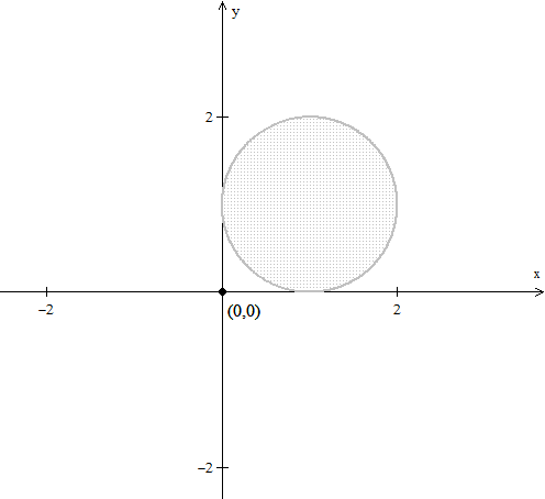
Find the maximum and minimum of f(x,y) = x² + y² on the closed set D = { (x,y)|(x − 1)² + (y − 1)² ≤ 1} .

First we note that D is a closed and bounded set and f is continuou and defined on D. Hence a maximum and minimum occur at D.
We find our critical points first, that is [df/dx] = 2x = 0 which gives x = 0 and [df/dy] = 2y = 0 which gives y = 0.
Note that the point ( 0,0 ) is not in our region D.
We can use Lagrange multipliers to find the maximum or minimum at the boundary g:(x − 1)² + (y − 1)² − 1 = 0.
Then
∇f = l∇g
g(x,y) = 0
is
(2x,2y) = l( 2(x − 1),2(y − 1) )
(x − 1)² + (y − 1)² − 1 = 0
and (2x,2y) = l( 2(x − 1),2(y − 1) ) is equivalent to
2x = 2l(x − 1)
2y = 2l(y − 1)
so our complete system of equations is
x = l(x − 1)
y = l(y − 1)
(x − 1)² + (y − 1)² − 1 = 0
Now, x0 or y0 as x = [l/(l − 1)] and y = [l/(l − 1)] and so x = y. Utilizing (x − 1)² + (y − 1)² − 1 = 0 we obtain 2(x − 1)² = 1 so x = 1 ±[1/(√2 )].
We have our possible extrema at f( 1 + [1/(√2 )],1 + [1/(√2 )] ) = [3/2] + [2/(√2 )] and f( 1 − [1/(√2 )],1 − [1/(√2 )] ) = [3/2] − [2/(√2 )].

Hence [3/2] + [2/(√2 )] is our maximum and [3/2] − [2/(√2 )] is our minimum.

Find the maximum and minimum of f(x,y) = 5x − y on the closed set D = { (x,y)| − 1 ≤ x ≤ 1, − 1 ≤ y ≤ 1} .

First we note that D is a closed and bounded set and f is continuous and defined on D. Hence a maximum and minimum occur at D.
We find our critical points first, that is [df/dx] = 5 = 0 which gives 5 = 0 and [df/dy] = − 1 = 0 which gives − 1 = 0 both which are not possible. Our extrema are located at the boundary.
We note that f is an increasing plane and so our maximum and minimum are achieved at the endpoinst of D.
Our possible extrema are then f( − 1, − 1) = − 4, f(1, − 1) = 6, f(1,1) = 4, f( − 1,1) = − 6.

Hence 6 is our maximum and − 6 is our minimum.

Find the point at the surface of x² + y² + z² = 1 closest and farthest to the point (3, − 1,2).

Recall that the distance from two points (x,y,z) and (3, − 1,2) in space is d(x,y,z) = √{(x − 3)² + (y + 1)² + (z − 2)²} .
We can use Lagrange multipliers to find the least or greatest distance, f:√{(x − 3)² + (y + 1)² + (z − 2)²} = 0 from a point in g:x² + y² + z² − 1 = 0 to the origin, that is subject to g.
Note that √{(x − 3)² + (y + 1)² + (z − 2)²} = 0 is equivalent to (x − 3)² + (y + 1)² + (z − 2)² = 0. Now
∇f = l∇g
g(x,y,z) = 0
is
(2(x − 3),2(y + 1),2(z − 2)) = l(2x,2y,2z)
x² + y² + z² − 1 = 0
(2(x − 3),2(y + 1),2(z − 2)) = l(2x,2y,2z) is equivalent to
x − 3 = xl
y + 1 = yl
z − 2 = zl
, note that x0, y0, and z0 as x − 3 = xl yields x = [3/(1 − l)], y + 1 = yl yields y = [( − 1)/(1 − l)] and z − 2 = zl yields z = [2/(1 − l)].
Utilizing x² + y² + z² − 1 = 0 we can substitute and obtain ( [3/(1 − l)] )² + ( [( − 1)/(1 − l)] )² + ( [2/(1 − l)] )² = 1 to solve for l and get l = 1 ±√{14} .
Then for l = 1 + √{14} we have x = [3/(1 − l)] = [3/(1 − (1 + √{14} ))] = [3/(√{14} )], y = [( − 1)/(1 − l)] = [( − 1)/(1 − (1 + √{14} ))] = [( − 1)/(√{14} )] and z = [2/(1 − l)] = [2/(1 − (1 + √{14} ))] = [2/(√{14} )].
Similarly for l = 1 − √{14} we have x = [3/(1 − l)] = [3/(1 − (1 − √{14} ))] = [3/( − √{14} )], y = [( − 1)/(1 − l)] = [( − 1)/(1 − (1 − √{14} ))] = [1/(√{14} )] and z = [2/(1 − l)] = [2/(1 − (1 − √{14} ))] = [2/( − √{14} )].
Then our value points are f( [3/(√{14} )], − [1/(√{14} )],[2/(√{14} )] ) ≈ 1.82 and f( − [3/(√{14} )],[1/(√{14} )], − [2/(√{14} )] ) ≈ 4.74

Thus our closest point on x² + y² + z² = 1 to (3, − 1,2) is ( [3/(√{14} )], − [1/(√{14} )],[2/(√{14} )] ) while the furthest is ( − [3/(√{14} )],[1/(√{14} )], − [2/(√{14} )] ).

« Previous Question | Next Question »

*These practice questions are only helpful when you work on them offline on a piece of paper and then use the solution steps function to check your answer.

Answer

More Lagrange Multiplier Examples

Lecture Slides are screen-captured images of important points in the lecture. Students can download and print out these lecture slide images to do practice problems as well as take notes while watching the lecture.

Intro

Example 1: Find the Point on the Surface z² -xy = 1 Closet to the Origin

Example 2: Find the Max & Min of f(x,y) = x² + 2y - x on the Closed Disc of Radius 1 Centered at the Origin

Intro 0:00
Example 1: Find the Point on the Surface z² -xy = 1 Closet to the Origin 0:54

Part 1
Part 2
Part 3

Example 2: Find the Max & Min of f(x,y) = x² + 2y - x on the Closed Disc of Radius 1 Centered at the Origin 16:05

Part 1
Part 2
Part 3

Multivariable Calculus

Section 1: Vectors
	Points & Vectors	28:23
	Scalar Product & Norm	30:25
	More on Vectors & Norms	38:18
	Inequalities & Parametric Lines	33:19
	Planes	29:59
	More on Planes	34:18
Section 2: Differentiation of Vectors
	Maps, Curves & Parameterizations	29:48
	Differentiation of Vectors	39:40
Section 3: Functions of Several Variables
	Functions of Several Variable	29:31
	Partial Derivatives	23:31
	Higher and Mixed Partial Derivatives	30:48
Section 4: Chain Rule and The Gradient
	The Chain Rule	28:03
	Tangent Plane	42:25
	Further Examples with Gradients & Tangents	47:11
	Directional Derivative	41:22
	A Unified View of Derivatives for Mappings	39:41
Section 5: Maxima and Minima
	Maxima & Minima	36:41
	Further Examples with Extrema	32:48
	Lagrange Multipliers	32:32
	More Lagrange Multiplier Examples	27:42
	Lagrange Multipliers, Continued	31:47
Section 6: Line Integrals and Potential Functions
	Line Integrals	36:08
	More on Line Integrals	28:04
	Line Integrals, Part 3	29:30
	Potential Functions	40:19
	Potential Functions, Continued	31:45
	Potential Functions, Conclusion & Summary	28:22
Section 7: Double Integrals
	Double Integrals	29:46
	Polar Coordinates	36:17
	Green's Theorem	38:01
	Divergence & Curl of a Vector Field	37:16
	Divergence & Curl, Continued	33:07
	Final Comments on Divergence & Curl	16:49
Section 8: Triple Integrals
	Triple Integrals	27:24
	Cylindrical & Spherical Coordinates	35:33
Section 9: Surface Integrals and Stokes' Theorem
	Parameterizing Surfaces & Cross Product	41:29
	Tangent Plane & Normal Vector to a Surface	37:06
	Surface Area	32:48
	Surface Integrals	46:52
	Divergence & Curl in 3-Space	23:40
	Divergence Theorem in 3-Space	34:12
	Stokes' Theorem, Part 1	22:01
	Stokes' Theorem, Part 2	20:32

Transcription: More Lagrange Multiplier Examples

Hello and welcome back to educator.com and Multivariable Calculus.0000

So, the last lesson, we introduced the method of Lagrange multipliers, we did a couple of basic examples.0004

In this lesson, we are just going to continue doing examples to develop a sense of how to handle this method of Lagrange multipliers.0009

Again, there is nothing particularly difficult about the method, it is pretty straight-forward. The difficulty is solving the simultaneous equations.0018

Because there is a lot going on, on the page, there are different cases when this equals 0, when this does not equal 0... so there are lots of things to keep track of.0025

These examples are going to be slightly more complicated, they are going to be handled the same way, they are just going to look like there is a lot more going on.0036

In some sense that is true, in some sense that is just the nature of Lagrange multiplier problems.0045

In any case, let us just jump right on in and see what we can do.0051

Okay. So, the first example. Example 1.0057

Find the point on the surface z² - xy = 1, closest to the origin.0065

Notice in this particular problem, they only gave us 1 function, and they just said closest to the origin.0090

This is an example of a Lagrange multiplier or a max/min problem where we have to extract information, come up with another function for ourselves whether it is f or g, depending on which one.0097

Right now, we are not quite sure which one is f and which one is g. So, find the point on the surface closest to the origin.0107

Well, distance from the origin is just the distance function. So, distance... I will write it out, that is not a problem... so distance = x² + y² + z², all under the radical.0116

As it turns out, we want the point that is closest to the origin, but the point has to be on this surface.0134

As it turns out, this is f, right here, and this is g. That is the constraint. We want to minimize, in other words, this function subject to this constraint.0144

Well, fortunately, since we are dealing with the distance function, if we minimize this square root function, it is the same as... we can also minimize the square of that: x² + y² + z².0156

I do not want to deal with the square root, so I will just instead of minimizing this, I am just going to minimize the function.0170

This is actually going to be my f, right here, and this is going to be my g.0176

Let us go ahead and form what it is that we actually form. We want to form the gradient of f, we want to set it equal to λ × the gradient of g, λ is our Lagrange multiplier.0184

Again, so we are going to have this set of equations and our constraint, which is going to be z² - xy - 1 = 0.0203

It is always going to be the constraint as a function set equal to 0. That is our other equation.0213

Now, we have to satisfy all of these simultaneously. Okay, let us just go ahead and take care of this.0222

So, the gradient of f, let us see... gradient of f, that is equal to... well, gradient of f is going to be 2x, 2y, and 2z.0230

That is going to equal... actually, let us just go ahead and do the gradient separately and then we will set it equal to each other.0245

The gradient of g is going to equal -y, that is df/dx, -x, that is df/dy, and 2z, that is df/dz of g.0255

Now, we set them equal to each other with the λ, so what we have is 2x, 2y, 2z is equal to... let me do this systematically, I do not want to get too far ahead of myself here... λ × -y, -x and 2z, which is equal to -λx, -λy, and 2λz.0268

Okay. There we go. Now, let us go to blue. This and that is one equation, this and that is another equation, this and that is a third equation, and of course we have our fourth equation. Those are our four equations and four unknowns, x, y, z, and λ.0306

Again, four equations and four unknowns. It is a bit much, but hopefully we should be able to work it out.0320

Let us see what we have got. One thing that we want... let me actually write out the equations here so that we have them in front of us... so, 2x = -λx... I am sorry, oops, I got these reversed, my apologies... this is -y, so this is y and this is x. There we go, that is a little bit better.0328

So, 2x = -λy. There you go, you can see it is very, very easy to go astray in these problems if you are not keeping track of every little thing.0359

So, -y and then we have 2y = -λx, and we have 2z = λ × 2z. Let us go ahead and actually write the other equation... z² - xy - 1 = 0.0374

Those are our four equations. Okay. So, let us just take a look at this for a second, and see how to proceed. One of the possibilities here is... well, one thing we know, we know that λ is not going to be 0. Let us exclude this possibility.0395

λ is definitely not going to be 0 because this would imply, if λ is 0, that means 2x = 0, 2y = 0, 2z = 0, because that would imply that x, y, and z equals 0, 0, 0, but 0, 0, 0, does not satisfy this equation.0413

If I put 0's in for here, what I get is -1 = 0, which is not true, so this particular point, if λ = 0, this particular point might work, but it does not satisfy the constraint. We can eliminate that as a possibility.0439

So that is good, λ is not equal to 0. So, our first possibility is... let me see, let us go ahead and move to the next page and let me rewrite the equation so that we have it above us.0454

So, 2x = -λy, 2y = λx, 2z = 2λz, and we have z² - xy - 1 = 0.0469

These are our four equations that we need to solve simultaneously. The one possibility here is let us take the possibility where z is not equal to 0. Okay.0490

So, when z is not equal to 0, that means we can go λ = 2z/2z, we solve this equation right over here, and we get λ = 1.0500

When λ = 1, I can put it into this equation and this equation. Then I get 2x = -y, and I get... I have 2y = -x.0519

Well, I am going to substitute one of these in here. I am going to take this, so I am going to rewrite this one as -2y = x, and I am going to substitute this x into that equation.0540

I get 2 × -2y = -y. I get -4y = y. and the only way that this is true, is that y = 0.0556

When y = 0, that means x = 0. Now, I have y = 0, and x = 0.0574

So, let us see here. That actually is a possibility, so now if y = 0 and x = 0, now let me go ahead and take these values and put them into this equation here.0590

Now I have got z² - 0 × 0 - 1 = 0, so I get z² = 1, I get z equals + or - 1.0605

My possibilities... so a couple of points, are (0,0,1), and (0,0,-1), right? x and y are 0, z is + or - 1.0622

Those are two possibilities. When I evaluate them at f, I end up with 1, and I end up with 1.0636

So, those are a couple of possibilities. This was the case when z was not equal to 0.0645

Now we will go ahead and do the case for z = 0, so we are just eliminating all of the possibilities here.0652

When z = 0, what we have is, if I take this equation, the constraint equation, I get 0² - xy - 1 = 0.0661

So, I get -xy = 1, or y = -1/x.0680

This is 1 relation that I have got here. Now, let me go back to my other relations involving x and y. That is 2x = -λ y, 2y = -λx.0690

I am going to divide the top and bottom equation, in other words I am going to divide the top equation by the bottom equation.0703

I get 2x/2y = -λy/-λx, the λ's cancel, and I get y/x.0712

So 2x/2y = y/x. The 2's actually end up cancelling, so I am just going to go ahead and cross multiply. I am going to get x² = y².0725

Well, let us see. x² = y², well I found that y = -1/x, therefore I am going to put this y into here and I am going to get x² = -1/x², which equals 1/x². That implies that x⁴ = 1.0741

Well, if x⁴ = 1, that implies that x = + or - 1.0768

When x = + or - 1, I go back to any one of the equations here, and I end up with y is equal to... well, let me actually move onto the next page here... so I have got x = + or - 1.0777

x = 1 implies that y = -1, and x = -1 implies that y = 1.0798

Now I have a couple of other points. z was 0, and these are the x's and y's.0812

One possibility is (1,-1,0), and the other possibility is (-1,1,0).0818

When I evaluate these at f, I get 2.0829

There we go. We have taken care of all of the possibilities. We had the four points, we had (0,0,1), (0,0,-1), and we have (1,-1,0), (-1,1,0).0841

For the other points, we found that the values were actually 1. Here the values are 2, so, the mins occur at (0,0,1) and (0,0,-1), and the value of the function at those points is 1.0855

On that given surface, on the surface z² - xy - 1 = 0, these 2 points on this surface are going to minimize the distance to the origin. That is what we have done here.0884

Again, as you can see, there seems to be a lot going on. Lots of cases to sort of go through. I wish that there was some sort of algorithmic approach to solving these problems other than the basic equation of setting the gradient of f = λ × gradient of g + the constraint equation equal to 0.0906

We have four equations and 4 unknowns, 5 equations and 5 unknowns. Clearly this gets more difficult. You just have lots of other cases to just sort of go through.0925

Again, successful Lagrange multipliers is more about experience than anything else. You can be reasonably systematic, but clearly you saw just with these 4 equations and 4 unknowns there is a lot to keep track of.0934

That is the only difficulty. Do not let the procedure actually interfere with your view of the mathematics.0949

Okay. Let us just do another example. That is all we can do, just keep doing examples until we start to get familiar with general notions. So, example number 2. Example 2.0958

Find the max and min of f(x,y) = x² + 2y² - x on the closed disc of radius 1 centered at the origin.0974

Okay. So, what we want to do is... we have the unit... now, we are considering the entire region, and it is a closed region. We are considering the interior and we are considering the boundary. That is all that is happening here.1016

So, let us see... equals 0... so this is the... our function, and we want to find the maximum and minimum values on this region.1035

We have a couple of things going on here. One of the things that we are going to do is... so this is kind of a max/min problem, and a Lagrange multiplier problem.1055

The Lagrange multiplier problem will usually apply to the boundary here, because we have an equation for that boundary which is x² + y² = 1, or x² + y² - 1 = 0.1072

As far as the interior is concerned, well we just treat it like any other max/min problem. We see if we can find a critical point and take it from there.1085

Let us go ahead and do that first. Let us deal with the interior, so, let us find the gradient of f and we will set it equal to 0 to see where the critical points are.1093

The gradient of f is going to be 2x - 1. That is the derivative with respect to the first variable x, and then we have 2y², I am sorry, this is 2y².1105

Our derivative with respect to y is going to be 4y. Okay. Now we want to check to see where these are equal to 0, so we have 2x - 1 = 0, and we have got 4y = 0.1123

This implies that y = 0 and this implies that x = 1/2, so at the point (1/2,0), the point (1/2,0) is a critical point.1136

Let us just go ahead and find the value of f at that point. When we go ahead and evaluate at that point, f(1/2,0), I go ahead and put it into f and I end up with -1/4.1154

That is one possible value. That is a critical point, that is on the interior. Now we can go ahead and deal with the boundary.1170

Now, let us check the boundary. So, the boundary is g(x,y) = x² + y² - 1, and that is going to be one of the equations, we will need to set that to 0.1180

Let us go ahead and find the gradient of g. The gradient of g is equal to, well that is going to be 2x, and that is going to be 2y.1195

So, 2x and 2y, so now we are going to go ahead and set the gradient of f = λ × gradient of g, and what we get is 2x - 1, and 4y = λ × 2x and 2y, which is equal 2λx and 2λy.1211

The two equations that we get are... let me do this one in red actually, so that I separate the equations out that I am going to be working on, again. This is all about solving simultaneous equations.1243

I get 2x = 2λx. I get 4y = 2λ × y. Let me make sure that I make everything clear so that we do not make the same mistake we made last time, so, this is 2λy.1254

And, of course we have our equation x² + y² - 1 = 0. That is the constraint.1273

Now I have got 3 equations and 3 unknowns, x, y, and λ.1280

So, let us deal with case 1. Case 1, let us take λ = 0.1286

So, case 1, λ = 0. Okay. When I set λ = 0, what is actually going to end up happening is I am just going to end up getting the previous answer.1297

That is not an issue, so let us deal with case 2.1309

case 2, where λ does not equal 0. So, one possibility for here, so, when λ does not equal to 0, now there are some sub cases that I have to consider.1315

The first sub case that I am going to consider is y = 0.1327

When I set y = 0, then I am going to get x² + 0² - 1 = 0. I am going to get x = + or - 1.1334

Therefore, I am going to have the points (1,0) and (-1,0).1349

Well, at (1,0), when I evaluate it at f, I am going to get 0, and when I evaluate it at (-1,0), when I evaluate f, I am going to get the value 2.1355

Now I have got (1,0), (-1,0), these are the values, and I also had that other point, that (1/2,0) that I found from just working on the interior of the disc and the value was I think -1/4, or something like that, or whatever it was.1370

Now, that is the case where λ does not = 0, and the case where y does equal 0. Now we want to consider the other case where y does not = 0.1385

Again, it seems like there is a lot going on but usually you can make sense of it by just spending some time with it. So, y does not equal 0.1400

Well, when y does not equal 0, 4y equals 2λ y. That means λ = 2. 4y/2y, let me go ahead and write that out actually. λ = 4y/2y = 2.1409

When λ = 2, this implies that 2x - 1 equals... so the equation is 2λx, right?1435

So 2x - 1 = λ = 2 = 4x, so I am going to get 2x = -1, x = -1/2.1454

So, when x = -1/2, now when I put that into my x² + y² - 1 = 0, when I put it into here, I am going to end up with the following.1469

It is going to be -1/2² + y² - 1 = 0.1491

I get 1/4 + y² - 1 = 0, I get y² = 3/4, therefore y = + or - sqrt(3)/2.1500

Okay, so, now my other points. x is -1/2, +sqrt(3)/2, and I get -1/2 - sqrt(3)/2.1516

When I evaluate these at f, I am going to end up with 9/4 and 9/4, so we have got 9/4, 9/4, -1/2, 0, I check all of those points to see which one is the maximum, which one is the minimum.1531

So the max takes place at the points (-1/2,sqrt(3)/2), and (-1/2,-sqrt(3)/2). Value is 9/4.1555

The minimum takes place at the original point that we found, which was... not -1/2... at 1/2, 0 and that value was -- let me see, what was that value if we can recall -- -1/4. There we go. This is our solution. I will go ahead and put f here, when we evaluate f.1580

So, at this point and this point, our function achieves a maximum and at this point, the function achieves a minimum. That is it.1610

Clearly there is a lot going on. A lot of things to sort of keep track of, but we are solving several equations in several variables. This is just the nature of the problem, the nature of the best.1618

Okay. So, in the next lesson, we are going to actually continue discussing Lagrange multipliers. We will do some more examples.1633

We will pull back a little bit so we will discuss some of the geometry of the solutions and we will try to make sense of what is actually going on.1640

Again, not theoretically, we just want this to seem reasonable to you, that we did not just drop this in your lap and say use this technique to find max/min for a function subject to this constraint. We still want this to make sense.1645

Okay. Thank you for joining us here at educator.com, we will see you next time. Bye-bye.1658

Related Books

Multivariable Calculus by Stewart, 7th Edition

Author: James Stewart

ISBN: 538497815

Publisher: Brooks Cole

Year: 2011

The book is filled with clear and accurate descriptions of concepts and is also has many relevant, real-world examples.

Related Books

Name	Description	Link
BookRenter.com	BookRenter.com is simply the most reliable online textbook rental service.	Visit BookRenter.com
PhysicsForums.com Homework Help	Physics Forums is a scientific community for students looking for math & science help.	Visit PhysicsForums.com Homework Help

Multivariable Calculus More Lagrange Multiplier Examples

Share this knowledge with your friends!

Copy & Paste this embed code into your website’s HTML

Discussion

Answer Engine

Practice Questions

Download Lecture Slides

Table of Contents

Transcription

Related Books

Answer EngineGet answers to any question!Ask any question related to Multivariable Calculus

More Lagrange Multiplier Examples

More Lagrange Multiplier Examples

Multivariable Calculus

Transcription: More Lagrange Multiplier Examples

Related Books

Related Books

Start Learning Now

Membership Overview

Multivariable Calculus More Lagrange Multiplier Examples

Share this knowledge with your friends!

Copy & Paste this embed code into your website’s HTML

Discussion

Answer Engine

Practice Questions

Download Lecture Slides

Table of Contents

Transcription

Related Books

Answer EngineGet answers to any question!Ask any question related to Multivariable Calculus

More Lagrange Multiplier Examples

More Lagrange Multiplier Examples

Multivariable Calculus

Transcription: More Lagrange Multiplier Examples

Related Books

Related Books

Available 24/7. Unlimited Access to Our Entire Library.

Searchable Lessons

Get Answers & Community Support

Downloadable Lecture Notes

Study Guides, Worksheets and Extra Example Lessons

Start Learning Now

Membership Overview