Raffi Hovasapian

Raffi Hovasapian

Maxima & Minima

Slide Duration:

Table of Contents

Section 1: Vectors
Points & Vectors

28m 23s

Intro
0:00
Points and Vectors
1:02
A Point in a Plane
1:03
A Point in Space
3:14
Notation for a Space of a Given Space
6:34
Introduction to Vectors
9:51
Adding Vectors
14:51
Example 1
16:52
Properties of Vector Addition
18:24
Example 2
21:01
Two More Properties of Vector Addition
24:16
Multiplication of a Vector by a Constant
25:27
Scalar Product & Norm

30m 25s

Intro
0:00
Scalar Product and Norm
1:05
Introduction to Scalar Product
1:06
Example 1
3:21
Properties of Scalar Product
6:14
Definition: Orthogonal
11:41
Example 2: Orthogonal
14:19
Definition: Norm of a Vector
15:30
Example 3
19:37
Distance Between Two Vectors
22:05
Example 4
27:19
More on Vectors & Norms

38m 18s

Intro
0:00
More on Vectors and Norms
0:38
Open Disc
0:39
Close Disc
3:14
Open Ball, Closed Ball, and the Sphere
5:22
Property and Definition of Unit Vector
7:16
Example 1
14:04
Three Special Unit Vectors
17:24
General Pythagorean Theorem
19:44
Projection
23:00
Example 2
28:35
Example 3
35:54
Inequalities & Parametric Lines

33m 19s

Intro
0:00
Inequalities and Parametric Lines
0:30
Starting Example
0:31
Theorem 1
5:10
Theorem 2
7:22
Definition 1: Parametric Equation of a Straight Line
10:16
Definition 2
17:38
Example 1
21:19
Example 2
25:20
Planes

29m 59s

Intro
0:00
Planes
0:18
Definition 1
0:19
Example 1
7:04
Example 2
12:45
General Definitions and Properties: 2 Vectors are Said to Be Paralleled If
14:50
Example 3
16:44
Example 4
20:17
More on Planes

34m 18s

Intro
0:00
More on Planes
0:25
Example 1
0:26
Distance From Some Point in Space to a Given Plane: Derivation
10:12
Final Formula for Distance
21:20
Example 2
23:09
Example 3: Part 1
26:56
Example 3: Part 2
31:46
Section 2: Differentiation of Vectors
Maps, Curves & Parameterizations

29m 48s

Intro
0:00
Maps, Curves and Parameterizations
1:10
Recall
1:11
Looking at y = x2 or f(x) = x2
2:23
Departure Space & Arrival Space
7:01
Looking at a 'Function' from ℝ to ℝ2
10:36
Example 1
14:50
Definition 1: Parameterized Curve
17:33
Example 2
21:56
Example 3
25:16
Differentiation of Vectors

39m 40s

Intro
0:00
Differentiation of Vectors
0:18
Example 1
0:19
Definition 1: Velocity of a Curve
1:45
Line Tangent to a Curve
6:10
Example 2
7:40
Definition 2: Speed of a Curve
12:18
Example 3
13:53
Definition 3: Acceleration Vector
16:37
Two Definitions for the Scalar Part of Acceleration
17:22
Rules for Differentiating Vectors: 1
19:52
Rules for Differentiating Vectors: 2
21:28
Rules for Differentiating Vectors: 3
22:03
Rules for Differentiating Vectors: 4
24:14
Example 4
26:57
Section 3: Functions of Several Variables
Functions of Several Variable

29m 31s

Intro
0:00
Length of a Curve in Space
0:25
Definition 1: Length of a Curve in Space
0:26
Extended Form
2:06
Example 1
3:40
Example 2
6:28
Functions of Several Variable
8:55
Functions of Several Variable
8:56
General Examples
11:11
Graph by Plotting
13:00
Example 1
16:31
Definition 1
18:33
Example 2
22:15
Equipotential Surfaces
25:27
Isothermal Surfaces
27:30
Partial Derivatives

23m 31s

Intro
0:00
Partial Derivatives
0:19
Example 1
0:20
Example 2
5:30
Example 3
7:48
Example 4
9:19
Definition 1
12:19
Example 5
14:24
Example 6
16:14
Notation and Properties for Gradient
20:26
Higher and Mixed Partial Derivatives

30m 48s

Intro
0:00
Higher and Mixed Partial Derivatives
0:45
Definition 1: Open Set
0:46
Notation: Partial Derivatives
5:39
Example 1
12:00
Theorem 1
14:25
Now Consider a Function of Three Variables
16:50
Example 2
20:09
Caution
23:16
Example 3
25:42
Section 4: Chain Rule and The Gradient
The Chain Rule

28m 3s

Intro
0:00
The Chain Rule
0:45
Conceptual Example
0:46
Example 1
5:10
The Chain Rule
10:11
Example 2: Part 1
19:06
Example 2: Part 2 - Solving Directly
25:26
Tangent Plane

42m 25s

Intro
0:00
Tangent Plane
1:02
Tangent Plane Part 1
1:03
Tangent Plane Part 2
10:00
Tangent Plane Part 3
18:18
Tangent Plane Part 4
21:18
Definition 1: Tangent Plane to a Surface
27:46
Example 1: Find the Equation of the Plane Tangent to the Surface
31:18
Example 2: Find the Tangent Line to the Curve
36:54
Further Examples with Gradients & Tangents

47m 11s

Intro
0:00
Example 1: Parametric Equation for the Line Tangent to the Curve of Two Intersecting Surfaces
0:41
Part 1: Question
0:42
Part 2: When Two Surfaces in ℝ3 Intersect
4:31
Part 3: Diagrams
7:36
Part 4: Solution
12:10
Part 5: Diagram of Final Answer
23:52
Example 2: Gradients & Composite Functions
26:42
Part 1: Question
26:43
Part 2: Solution
29:21
Example 3: Cos of the Angle Between the Surfaces
39:20
Part 1: Question
39:21
Part 2: Definition of Angle Between Two Surfaces
41:04
Part 3: Solution
42:39
Directional Derivative

41m 22s

Intro
0:00
Directional Derivative
0:10
Rate of Change & Direction Overview
0:11
Rate of Change : Function of Two Variables
4:32
Directional Derivative
10:13
Example 1
18:26
Examining Gradient of f(p) ∙ A When A is a Unit Vector
25:30
Directional Derivative of f(p)
31:03
Norm of the Gradient f(p)
33:23
Example 2
34:53
A Unified View of Derivatives for Mappings

39m 41s

Intro
0:00
A Unified View of Derivatives for Mappings
1:29
Derivatives for Mappings
1:30
Example 1
5:46
Example 2
8:25
Example 3
12:08
Example 4
14:35
Derivative for Mappings of Composite Function
17:47
Example 5
22:15
Example 6
28:42
Section 5: Maxima and Minima
Maxima & Minima

36m 41s

Intro
0:00
Maxima and Minima
0:35
Definition 1: Critical Point
0:36
Example 1: Find the Critical Values
2:48
Definition 2: Local Max & Local Min
10:03
Theorem 1
14:10
Example 2: Local Max, Min, and Extreme
18:28
Definition 3: Boundary Point
27:00
Definition 4: Closed Set
29:50
Definition 5: Bounded Set
31:32
Theorem 2
33:34
Further Examples with Extrema

32m 48s

Intro
0:00
Further Example with Extrema
1:02
Example 1: Max and Min Values of f on the Square
1:03
Example 2: Find the Extreme for f(x,y) = x² + 2y² - x
10:44
Example 3: Max and Min Value of f(x,y) = (x²+ y²)⁻¹ in the Region (x -2)²+ y² ≤ 1
17:20
Lagrange Multipliers

32m 32s

Intro
0:00
Lagrange Multipliers
1:13
Theorem 1
1:14
Method
6:35
Example 1: Find the Largest and Smallest Values that f Achieves Subject to g
9:14
Example 2: Find the Max & Min Values of f(x,y)= 3x + 4y on the Circle x² + y² = 1
22:18
More Lagrange Multiplier Examples

27m 42s

Intro
0:00
Example 1: Find the Point on the Surface z² -xy = 1 Closet to the Origin
0:54
Part 1
0:55
Part 2
7:37
Part 3
10:44
Example 2: Find the Max & Min of f(x,y) = x² + 2y - x on the Closed Disc of Radius 1 Centered at the Origin
16:05
Part 1
16:06
Part 2
19:33
Part 3
23:17
Lagrange Multipliers, Continued

31m 47s

Intro
0:00
Lagrange Multipliers
0:42
First Example of Lesson 20
0:44
Let's Look at This Geometrically
3:12
Example 1: Lagrange Multiplier Problem with 2 Constraints
8:42
Part 1: Question
8:43
Part 2: What We Have to Solve
15:13
Part 3: Case 1
20:49
Part 4: Case 2
22:59
Part 5: Final Solution
25:45
Section 6: Line Integrals and Potential Functions
Line Integrals

36m 8s

Intro
0:00
Line Integrals
0:18
Introduction to Line Integrals
0:19
Definition 1: Vector Field
3:57
Example 1
5:46
Example 2: Gradient Operator & Vector Field
8:06
Example 3
12:19
Vector Field, Curve in Space & Line Integrals
14:07
Definition 2: F(C(t)) ∙ C'(t) is a Function of t
17:45
Example 4
18:10
Definition 3: Line Integrals
20:21
Example 5
25:00
Example 6
30:33
More on Line Integrals

28m 4s

Intro
0:00
More on Line Integrals
0:10
Line Integrals Notation
0:11
Curve Given in Non-parameterized Way: In General
4:34
Curve Given in Non-parameterized Way: For the Circle of Radius r
6:07
Curve Given in Non-parameterized Way: For a Straight Line Segment Between P & Q
6:32
The Integral is Independent of the Parameterization Chosen
7:17
Example 1: Find the Integral on the Ellipse Centered at the Origin
9:18
Example 2: Find the Integral of the Vector Field
16:26
Discussion of Result and Vector Field for Example 2
23:52
Graphical Example
26:03
Line Integrals, Part 3

29m 30s

Intro
0:00
Line Integrals
0:12
Piecewise Continuous Path
0:13
Closed Path
1:47
Example 1: Find the Integral
3:50
The Reverse Path
14:14
Theorem 1
16:18
Parameterization for the Reverse Path
17:24
Example 2
18:50
Line Integrals of Functions on ℝn
21:36
Example 3
24:20
Potential Functions

40m 19s

Intro
0:00
Potential Functions
0:08
Definition 1: Potential Functions
0:09
Definition 2: An Open Set S is Called Connected if…
5:52
Theorem 1
8:19
Existence of a Potential Function
11:04
Theorem 2
18:06
Example 1
22:18
Contrapositive and Positive Form of the Theorem
28:02
The Converse is Not Generally True
30:59
Our Theorem
32:55
Compare the n-th Term Test for Divergence of an Infinite Series
36:00
So for Our Theorem
38:16
Potential Functions, Continued

31m 45s

Intro
0:00
Potential Functions
0:52
Theorem 1
0:53
Example 1
4:00
Theorem in 3-Space
14:07
Example 2
17:53
Example 3
24:07
Potential Functions, Conclusion & Summary

28m 22s

Intro
0:00
Potential Functions
0:16
Theorem 1
0:17
In Other Words
3:25
Corollary
5:22
Example 1
7:45
Theorem 2
11:34
Summary on Potential Functions 1
15:32
Summary on Potential Functions 2
17:26
Summary on Potential Functions 3
18:43
Case 1
19:24
Case 2
20:48
Case 3
21:35
Example 2
23:59
Section 7: Double Integrals
Double Integrals

29m 46s

Intro
0:00
Double Integrals
0:52
Introduction to Double Integrals
0:53
Function with Two Variables
3:39
Example 1: Find the Integral of xy³ over the Region x ϵ[1,2] & y ϵ[4,6]
9:42
Example 2: f(x,y) = x²y & R be the Region Such That x ϵ[2,3] & x² ≤ y ≤ x³
15:07
Example 3: f(x,y) = 4xy over the Region Bounded by y= 0, y= x, and y= -x+3
19:20
Polar Coordinates

36m 17s

Intro
0:00
Polar Coordinates
0:50
Polar Coordinates
0:51
Example 1: Let (x,y) = (6,√6), Convert to Polar Coordinates
3:24
Example 2: Express the Circle (x-2)² + y² = 4 in Polar Form.
5:46
Graphing Function in Polar Form.
10:02
Converting a Region in the xy-plane to Polar Coordinates
14:14
Example 3: Find the Integral over the Region Bounded by the Semicircle
20:06
Example 4: Find the Integral over the Region
27:57
Example 5: Find the Integral of f(x,y) = x² over the Region Contained by r= 1 - cosθ
32:55
Green's Theorem

38m 1s

Intro
0:00
Green's Theorem
0:38
Introduction to Green's Theorem and Notations
0:39
Green's Theorem
3:17
Example 1: Find the Integral of the Vector Field around the Ellipse
8:30
Verifying Green's Theorem with Example 1
15:35
A More General Version of Green's Theorem
20:03
Example 2
22:59
Example 3
26:30
Example 4
32:05
Divergence & Curl of a Vector Field

37m 16s

Intro
0:00
Divergence & Curl of a Vector Field
0:18
Definitions: Divergence(F) & Curl(F)
0:19
Example 1: Evaluate Divergence(F) and Curl(F)
3:43
Properties of Divergence
9:24
Properties of Curl
12:24
Two Versions of Green's Theorem: Circulation - Curl
17:46
Two Versions of Green's Theorem: Flux Divergence
19:09
Circulation-Curl Part 1
20:08
Circulation-Curl Part 2
28:29
Example 2
32:06
Divergence & Curl, Continued

33m 7s

Intro
0:00
Divergence & Curl, Continued
0:24
Divergence Part 1
0:25
Divergence Part 2: Right Normal Vector and Left Normal Vector
5:28
Divergence Part 3
9:09
Divergence Part 4
13:51
Divergence Part 5
19:19
Example 1
23:40
Final Comments on Divergence & Curl

16m 49s

Intro
0:00
Final Comments on Divergence and Curl
0:37
Several Symbolic Representations for Green's Theorem
0:38
Circulation-Curl
9:44
Flux Divergence
11:02
Closing Comments on Divergence and Curl
15:04
Section 8: Triple Integrals
Triple Integrals

27m 24s

Intro
0:00
Triple Integrals
0:21
Example 1
2:01
Example 2
9:42
Example 3
15:25
Example 4
20:54
Cylindrical & Spherical Coordinates

35m 33s

Intro
0:00
Cylindrical and Spherical Coordinates
0:42
Cylindrical Coordinates
0:43
When Integrating Over a Region in 3-space, Upon Transformation the Triple Integral Becomes..
4:29
Example 1
6:27
The Cartesian Integral
15:00
Introduction to Spherical Coordinates
19:44
Reason It's Called Spherical Coordinates
22:49
Spherical Transformation
26:12
Example 2
29:23
Section 9: Surface Integrals and Stokes' Theorem
Parameterizing Surfaces & Cross Product

41m 29s

Intro
0:00
Parameterizing Surfaces
0:40
Describing a Line or a Curve Parametrically
0:41
Describing a Line or a Curve Parametrically: Example
1:52
Describing a Surface Parametrically
2:58
Describing a Surface Parametrically: Example
5:30
Recall: Parameterizations are not Unique
7:18
Example 1: Sphere of Radius R
8:22
Example 2: Another P for the Sphere of Radius R
10:52
This is True in General
13:35
Example 3: Paraboloid
15:05
Example 4: A Surface of Revolution around z-axis
18:10
Cross Product
23:15
Defining Cross Product
23:16
Example 5: Part 1
28:04
Example 5: Part 2 - Right Hand Rule
32:31
Example 6
37:20
Tangent Plane & Normal Vector to a Surface

37m 6s

Intro
0:00
Tangent Plane and Normal Vector to a Surface
0:35
Tangent Plane and Normal Vector to a Surface Part 1
0:36
Tangent Plane and Normal Vector to a Surface Part 2
5:22
Tangent Plane and Normal Vector to a Surface Part 3
13:42
Example 1: Question & Solution
17:59
Example 1: Illustrative Explanation of the Solution
28:37
Example 2: Question & Solution
30:55
Example 2: Illustrative Explanation of the Solution
35:10
Surface Area

32m 48s

Intro
0:00
Surface Area
0:27
Introduction to Surface Area
0:28
Given a Surface in 3-space and a Parameterization P
3:31
Defining Surface Area
7:46
Curve Length
10:52
Example 1: Find the Are of a Sphere of Radius R
15:03
Example 2: Find the Area of the Paraboloid z= x² + y² for 0 ≤ z ≤ 5
19:10
Example 2: Writing the Answer in Polar Coordinates
28:07
Surface Integrals

46m 52s

Intro
0:00
Surface Integrals
0:25
Introduction to Surface Integrals
0:26
General Integral for Surface Are of Any Parameterization
3:03
Integral of a Function Over a Surface
4:47
Example 1
9:53
Integral of a Vector Field Over a Surface
17:20
Example 2
22:15
Side Note: Be Very Careful
28:58
Example 3
30:42
Summary
43:57
Divergence & Curl in 3-Space

23m 40s

Intro
0:00
Divergence and Curl in 3-Space
0:26
Introduction to Divergence and Curl in 3-Space
0:27
Define: Divergence of F
2:50
Define: Curl of F
4:12
The Del Operator
6:25
Symbolically: Div(F)
9:03
Symbolically: Curl(F)
10:50
Example 1
14:07
Example 2
18:01
Divergence Theorem in 3-Space

34m 12s

Intro
0:00
Divergence Theorem in 3-Space
0:36
Green's Flux-Divergence
0:37
Divergence Theorem in 3-Space
3:34
Note: Closed Surface
6:43
Figure: Paraboloid
8:44
Example 1
12:13
Example 2
18:50
Recap for Surfaces: Introduction
27:50
Recap for Surfaces: Surface Area
29:16
Recap for Surfaces: Surface Integral of a Function
29:50
Recap for Surfaces: Surface Integral of a Vector Field
30:39
Recap for Surfaces: Divergence Theorem
32:32
Stokes' Theorem, Part 1

22m 1s

Intro
0:00
Stokes' Theorem
0:25
Recall Circulation-Curl Version of Green's Theorem
0:26
Constructing a Surface in 3-Space
2:26
Stokes' Theorem
5:34
Note on Curve and Vector Field in 3-Space
9:50
Example 1: Find the Circulation of F around the Curve
12:40
Part 1: Question
12:48
Part 2: Drawing the Figure
13:56
Part 3: Solution
16:08
Stokes' Theorem, Part 2

20m 32s

Intro
0:00
Example 1: Calculate the Boundary of the Surface and the Circulation of F around this Boundary
0:30
Part 1: Question
0:31
Part 2: Drawing the Figure
2:02
Part 3: Solution
5:24
Example 2: Calculate the Boundary of the Surface and the Circulation of F around this Boundary
13:11
Part 1: Question
13:12
Part 2: Solution
13:56
Loading...
This is a quick preview of the lesson. For full access, please Log In or Sign up.
For more information, please see full course syllabus of Multivariable Calculus
Bookmark & Share Embed

Share this knowledge with your friends!

Copy & Paste this embed code into your website’s HTML

Please ensure that your website editor is in text mode when you paste the code.
(In Wordpress, the mode button is on the top right corner.)
  ×
  • - Allow users to view the embedded video in full-size.
Since this lesson is not free, only the preview will appear on your website.
  • Discussion

  • Answer Engine

  • Practice Questions

  • Download Lecture Slides

  • Table of Contents

  • Transcription

  • Related Books

Lecture Comments (2)

1 answer

Last reply by: Professor Hovasapian
Fri Aug 16, 2013 2:39 AM

Post by Frank Sui on August 15, 2013

Example 2, first one should be "Choose (2nπ,-1) w/ n=o So (0,-1)" instead of "(2nπ,1)", right?

Maxima & Minima

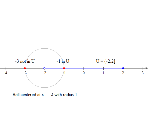
Consider the interval ( − 2,2] on the real line.
Determine if the following points are boudary points using a ball B of raidus 1 at each point.
i) x = − 2
  • A point P is a boundary point of a set U if an open ball using P as the center contains points in U and not in U.
An open ball centered at − 2 will contain all points in the interval [ − 3, − 1]. Note that − 3 ∉ ( − 2,2] and − 1 ∈ ( − 2,2], so x = − 2 is a boundary point. See image:
Consider the interval ( − 2,2] on the real line.
Determine if the following points are boudary points using a ball B of raidus 1 at each point.
ii) x = 2.5
  • A point P is a boundary point of a set U if an open ball using P as the center contains points in U and not in U.
An open ball centered at 2.5 will contain all points in the interval [1.5,3.5]. Note that 3 ∉ ( − 2,2] and 2 ∈ ( − 2,2], so x = 2.5 is a boundary point. Also 2.5 ∉ ( − 2,2], hence boundary points need not be part of our set.
Consider the interval ( − 2,2] on the real line.
Determine if the following points are boudary points using a ball B of raidus 1 at each point.
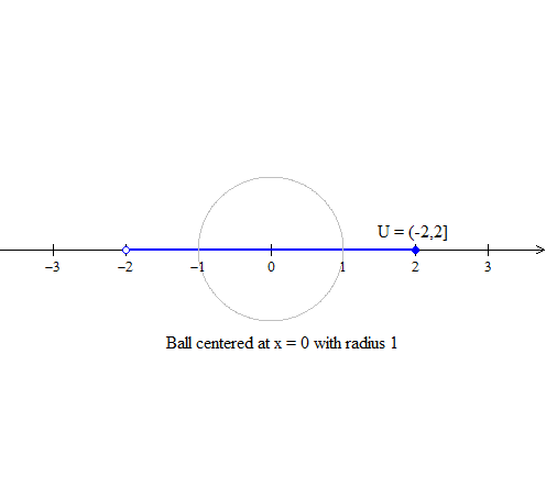
iii) x = 0
  • A point P is a boundary point of a set U if an open ball using P as the center contains points in U and not in U.
An open ball centered at 0 will contain all points in the interval [ − 1,1]. Note that this ball contains points in ( − 2,2] only, so x = 0 is not a boundary point. See image:
Consider the interval ( − 2,2] on the real line.
Determine if the following points are boudary points using a ball B of raidus 1 at each point.
iv) x = − 3
  • A point P is a boundary point of a set U if an open ball using P as the center contains points in U and not in U.
An open ball centered at − 3 will contain all points in the interval [ − 4, − 2]. Note that this ball contains no points in ( − 2,2], so x = − 3 is not a boundary point.
Determine whether the following sets are open, closed or neither.
i) { x| − 1 < x < 0}
A set is closed if it contains all of its boundary points, that is, the endpoints are part of the set. Clearly − 1 and 0 are not in the set, thus this set is open.
Determine whether the following sets are open, closed or neither.
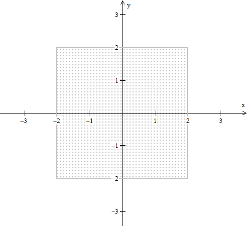
ii) { (x,y) - − 2 ≥ x ≥ 2, − 2 ≥ y ≥ 2}
A set is closed if it contains all of its boundary points, that is, the endpoints are part of the set. Note that this set is a square containing its boundary. Hence this set is closed. See image:
Determine whether the following sets are open, closed or neither.
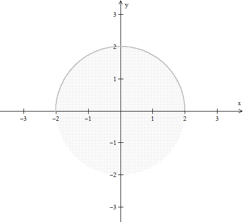
iii) { (x,y)|y ≥ √{4 − x2} ,y >− √{4 − x2} }
  • A set is closed if it contains all of its boundary points, that is, the endpoints are part of the set. Note that this is a circle whose lower half does not contain its boundary points while its top half does.
Hence this set is neither open or closed. See image:
i) Show that the set D1 = { x|0 ≥ x ≥ 1} is bounded.
  • A set is bounded if we can find a number N such that for every point x ∈ D1, || x || ≥ N.
  • Note that the norm is equivalent to the absolute value in one dimension. Since our set D2 has 1 as its maximum norm, we can choose N = 2 to show that D2 is bounded, as 1 < 2 = N.
  • ii) Show that the set D2 = { (x,y)|y = [1/x] } is not bounded.
  • Note that the points in D2 have no restriction aside x0. Hence we can not find a number N such that || (x,y) ||≥ N.
  • For instance (1,1) has norm √2 so N = 2 is sufficient but || ( 4,[1/4] ) ||> 2. Then N = 3 becomes sufficient but again || ( 9,[1/9] ) ||> 3, this pattern can go on infinetly.
Hence D2 is not bounded.
i) Let S1 = { x| − 1 ≥ x ≥ 1} . Find the local maxima and minima of the function y = x2 − 1 on S1.
  • Recall that a critical point is found by solving [dy/dx] = 0 for x. In our case we obtain 0 = 2x or x = 0.
  • Using the first derivative test we can see that at x = 0 we have a minimum, our point is (0, − 1).
  • We must also check our endpoints x = − 1 and x = 1 for they too can be extrema.
  • At x = − 0.9 ∈ S1 (slightly greater than − 1) we have the value − 0.19 while the value at x = − 1 is 0. From the left the function is clearly decreasing, so x = − 1 is a maximum.
  • At x = 0.9 ∈ S1 (slightly less than 1) we have the value − 0.19 while the value at x = 1 is 0. From x = 0 the function is now increasing, so x = 1 is a maximum.
We therefore have two maximum points ( − 1,0) and (1,0).
ii) Let S2 = { x| − 1 < x < 1} . Find the local maxima and minima of the function y = x2 − 1 on S2.
  • Note that our set is open, our only extrema might occur at our critical points.
In this case x = 0 is our only critical point, by the first derivative test we find that this is a minimum at (0, − 1).
Find all possible critical points for f(x,y) = 2x2 − y2.
  • For a function of two variables, the critical points occur where all first partial derivatives equal zero.
  • So [df/dx] = 4x and [df/dy] = − 2y. Now 4x = 0 yields x = 0 while − 2y = 0 yields y = 0.
Our critical point is f(0,0) = 0 or at (0,0,0).
Find all possible critical points for f(x,y) = exy.
  • For a function of two variables, the critical points occur where all first partial derivatives equal zero.
  • So [df/dx] = yexy and [df/dy] = xexy. Now yexy = 0 yields y = 0 or exy = 0 but exy0. Similarly xexy = 0 yields x = 0.
Our critical point is f(0,0) = 1 or at (0,0,1).
Find all possible critical points for f(x,y) = xsin(y).
  • For a function of two variables, the critical points occur where all first partial derivatives equal zero.
  • So [df/dx] = sin(y) and [df/dy] = xcos(y). Now sin(y) = 0 occurs at y = np for n = 0,1,2, … while xcos(y) = 0 yields x = 0 or cos(y) = 0 which occurs at y = [((2n + 1)p)/2] for n = 0,1,2 …
Our critical points are f(0,np) = 0 or at (0,np) and f( 0,[((2n + 1)p)/2] ) = 0 or at ( 0,[((2n + 1)p)/2] ) for n = 0,1,2, …
Check to see if the critical point (0,0,0) is a maximum, minimum or neither for f(x,y) = 2x2 − y2.
  • Note that for large values of x and small values of y, f(x,y) > 0. For instance f(10,1) = 199.
  • But for small values of x and large values of y, f(x,y) < 0. For instance f(1,10) = − 98.
Since − 98 < 0 < 199, that is (1,10, − 98) < (0,0,0) < (10,1,199), our critical point is neither a minimum nor a maximum.
Check to see if the critical point (0,0,1) is a maximum, minimum or neither for f(x,y) = exy.
  • Note that if x > 0 and y < 0, f(x,y) < 1. Similarly for x < 0 and y > 0.
  • Yet if both x > 0 and y > 0 or x < 0 and y < 0, f(x,y) > 1.
Since (0,0,1 lies in between these two, our critical point is neither a minimum nor a maximum.
Check to see if the critical point (0,p,0) is a maximum, minimum or neither for f(x,y) = xsin(y).
  • We can check two close points to (0,p,1) to determine if the critical point is an extrema.
  • Now, f(0.1,3.14) ≈ 0.00548 and f( − 0.1,3.14) ≈ − 0.00548.
Since f( − 0.1,3.14) < 0 < f(0.1,3.14) the critical point (0,p,1) is neither a minimum nor a maximum.

*These practice questions are only helpful when you work on them offline on a piece of paper and then use the solution steps function to check your answer.

Answer

Maxima & Minima

Lecture Slides are screen-captured images of important points in the lecture. Students can download and print out these lecture slide images to do practice problems as well as take notes while watching the lecture.

  • Intro 0:00
  • Maxima and Minima 0:35
    • Definition 1: Critical Point
    • Example 1: Find the Critical Values
    • Definition 2: Local Max & Local Min
    • Theorem 1
    • Example 2: Local Max, Min, and Extreme
    • Definition 3: Boundary Point
    • Definition 4: Closed Set
    • Definition 5: Bounded Set
    • Theorem 2

Transcription: Maxima & Minima

Hello and welcome back to educator.com and multi-variable calculus.0000

Today we are going to start out discussion of maxima and minima. Finding points in the domain where the function obtains a maximum and where it obtains a minimum, just like in single variable calculus.0004

So, a lot of the things you learned in single variable calculus are going to apply here.0016

Now, instead of one variable, x, you are going to have 2, 3, sometimes more.0020

So, the problems tend to become a little bit longer, a little bit more involved, but again it is still just a max, min problem based on the derivative. Let us just jump right on in.0026

Okay. So, let me see, let me go ahead and just write a... well, let us go ahead and start with a definition. How is that?0039

I think... we do not really need a preamble here, so let f be a differentiable function -- and again by differentiable we just mean well-behaved, it has a derivative, no problem, no worries, no concerns -- on an open set.0047

Again, you recall what an open set means. It is just a set that does not have boundary points. An open set u.0075

Let p be a point in u. p is called a critical point or a critical value, we will use both terms, it is called a critical point if each partial derivative evaluated at p is equal to 0.0085

So you see this is the exact definition as for single calculus. The derivative is equal to 0 at a critical point.0130

So, let us go ahead and write what this is symbolically. We will say that is di(f) = 0.0136

So, the first derivative, second derivative, third partial, fourth partial, whatever it is.0147

Or, df/dxi evaluated at p is equal to 0. Let me actually add one more thing here. It is very... evaluating it at p, so we will actually put the p in there.0153

So, that is it. Let us just do an example. Example 1. Find the critical values of f(x,y) = x + ysin(x).0169

Let us go ahead and find the derivatives. The partial with respect to x, df/dx = 1 + ycos(x), right? We are holding y as a constant.0196

The partial derivative with respect to y is going to equal just sin(x). This one is going to be held as a constant, the x goes to 0.0212

Let us see what we have got here. So, here, we want each of these, of course, equal to 0.0223

So 1 + ycos(x) = 0, and sin(x) = 0, so let us go ahead and do this one first.0231

sin(x) = 0, so our possible values of x are going to be 0, and π, and 2π, and 3π, and so on.0243

Now, let us see... should we do... yea, okay. Let us go ahead and take a particular value. Let us just take... so the 0, the 2π, the 4π, when we take the cosine of that, so now we are going to use these to actually solve for the y variable.0255

We have 0, 2π, 3π... I am sorry, 0, 2π, 4π, 6π, then we have the odds. π, 3π, 5π, so we have to check both possibilities because it turns out y is going to equal 2 different numbers.0281

So, let us go ahead and start with, let us say 2nπ, so when I take the evens, the 0, the 2, the 4, it is going to be... all of those can actually be written as x = 2nπ, where n is just some integer.0293

This little, funny-looking z here, that is a symbol for the integers. You know, integers, negative, 0, 1, 2, 3, 4, 5, that is it. Natural numbers including the negative versions of those negative numbers and 0.0313

This is a shorthand notation for writing the even number ones.0328

So, when we do that, we get 1 + y × cos(2nπ) = 0.0333

Well, cosine of any 2nπ, so 0, 2π, 4π, is the cosine of... it is going to be 1.0342

So you get 1 + y = 0, you are going to get y = -1.0351

Now we will go ahead and do the version for the odds. Well, the odds, the π, the 3π, the 5π and so on, that is going to be (2n+1)π.0357

That is the shorthand notation for all of the odds. Basically you just run n. So when n = 0, you have got π, when n = 1, you have got 3 π, when n = 2, you have got 5π. That is what this means.0370

So, when we do this one, we get... let me write it down here, that is okay... so we get 1 + y × cos(2n+1)π, and the cos((2n+1)π) for all n is going to be -1.0384

So what you end up with is 1 - y = 0, so y = 1.0406

So our final solution is going to look like this. Let us go ahead and write... yeah, we will write it on the next page.0415

So, the critical values are going to be all of the points 2nπ - 1, and 2n + 1π, 1, in other words the x value is going to be 2n + 1π, and the y value is going to be 1.0423

This is for n in z, where n is any integer at all, so we have 2 different possibilities.0448

That is it. It is that simple, you just take the partial derivatives, you set them equal to 0, and now instead of just having the one equation that you solve, you are going to have 2, 3, 4, however many equations and you just have to find all of the different values.0456

You are just going to have a lot of values, so you might have one critical value.0469

It just depends. You have to use all of the resources at your disposal, all of the things you know about a function, whether it is its graph, whether it is its particular behavior, whether it is a certain limit approaching something to come up with what these critical values are.0475

So, let us go ahead and speak about the critical values a little bit. The critical values for a function need not be local max's or min's.0492

You remember from first variable calculus, just because you find a critical value, some place where the derivative equals 0, that does not necessarily mean that it is a local max or a local min.0522

There are situations where it is neither, where it is an inflection point. So, the same thing can happen here, you know in several variables. It does not have to be a local max or min, it just means that it might be.0532

We have to subject the function to further analysis, to see if it is a local max or min, and later on if we are dealing with a closed domain if it is an absolute max or min. That is what is happening.0542

So, recall, we can have f'(x) = 0 and have a point of inflection, which is neither max nor min.0556

It looks something like this. So the graph comes like this, but you get a derivative of 0, so this point right here, I mean yeah, its derivative is 0, it is a horizontal slope, but the horizontal slope... but it is not a max or min, it is a point of inflection. That is a possibility too.0589

So, let us start with another definition here. Let f be a function on an open set u, a point p... and again these definitions, you know what they are... but again, we want to be reasonably formal in mathematics.0605

A point p is a local max for the function, if... oops, let us erase that... if there is an open ball -- and I will draw a picture in a minute -- centered at p such that f(x) < or = to f(p) for all x in that ball.0638

Let us go ahead and think about what this means. So in this particular... this is a general definition, it works in any number of dimensions.0696

So, the example I am going to use to demonstrate it is going to be in R2, in the plane, because that is the one that we are the most familiar with.0704

So, in R2, it looks like this. It looks like... so we have R2, and we have our point p... now an open ball around point p, centered at p, in this case is just an open disc.0710

If you are dealing in 3 dimensions, then you are talking about a point and there is an open ball. An open ball means, again, the boundary points are not included.0730

It is just some region around it, that you are not specifying a boundary on it.0737

Basically it says for any x-value, in here, for any x-value that I pick around that point, if a function, if I evaluate the function at any of the x's, at any point that I pick in that open ball, if all of them are less than or equal to the value of the function at p, then that is a local max.0742

So, the graph of this, of course, if you... so if your domain is 2 dimensions, so here we are talking about a function from R2 to R.0766

So, this is our domain, we are picking points from here, we are sticking it in a function, we are doing something to it, we are spitting out a number. That number is used as the z coordinate.0776

So, a function from R2 to R, actually gives you a surface in 3-space. So if this is the domain, there is some surface on top. It is just saying that what you have is something like that.0786

That here is the point, and then every point around p forms some sort of a, like a, cone or something. It is a local maximum, not an absolute maximum because we are talking about an open domain.0795

In a minute we will actually define what we mean by absolute max and closed domains.0808

So, that is it. Again, exactly the same as first variable calculus, or single variable calculus.0812

So, let us just go ahead and formalize one last thing. So, a local min is defined the same way.0820

It is defined the same way except of course all of the functional values are > or = f(p).0830

So, you have something that looks like this where p is down here, and all of the values around it are bigger than that.0843

Let us go ahead and write down a theorem. Now, let f be a function defined, and differentiable on an open set u, and let p be a local extremum.0851

An extremum is just a single word that takes care of both max and min at the same time. So extremum, plural being extrema. So it is max or min.0894

Let p be a local extremum for f on u. Then p is a critical point.0911

This is really, really important here. This is saying that if p happens to be a local max or min, that means that it is a critical point.0924

It does not mean... this theorem does not say that if p is a critical point, then it is a local max or min, because we know that that is not true.0934

The implication only works in one direction, not the other. Let me write this out.0944

So, note, a local extremum implies a critical point -- this double arrow in mathematics means implies -- not, definitely not. It does not mean it goes the other way. It does not mean if it is a critical point, it is a local extremum.0949

This is a very important point of logic in mathematics. Most implications -- not most, many implications only work in one direction, and we have to be very, very clear that we are not just automatically assuming that it works in the other direction.0973

Critical point does not imply a local extremum. This is not true.0990

However, what is true is something called a contrapositive of this. A local extremum implies that it is a critical point.1001

What is also true is that if it is not a critical point, then it is not a local extremum.1011

So, a implies b is the same as not b implying not a.1018

The way theorems are actually written in mathematics, it is often the case that we do not use them as written. We often use them in another form.1029

This is one of the ones where we often use in the other direction, because when we are given a function, we actually do not know whether it is a local max or min, to decide whether it is a critical value. We are working in the other direction.1038

We are actually looking at the function and finding the derivative and the partial derivatives, and setting them equal to 0. We are finding points that are critical values and then we are checking to see if they are local max's or min's.1050

What we can say, what this theorem does allow us to say, is that if I find, if I take the derivatives of functions, set them equal to 0 and realize there is no value in the domain, x or y, there is no point x or y where the derivative = 0, then there is no local max or min.1061

That is what is going on here. In this case, the theorem is written as if -- you know -- p is a local max or min, then it is a critical point.1080

Often, how we will be using it is if it is not a critical point, then it is not a local max or min. We will be using the contra-positive of that.1088

So, if a implies b, that is the same as not b implying not a. That is very, very important.1097

Let us go ahead and do an example here. Example 2.1105

Let us check to see if the critical values of Example 1 are local extremum, or local max's or min's.1118

So, again, just because they are critical values, that is not a guarantee, we have to see if they are local max's or min's.1145

So we had the fact that f(x,y) = x + y × sin(x).1151

We had critical values -- what is with my h's here? -- We had critical values of (2nπ,-1) and (2n + 1π,1).1169

Defined for all n in z integers, so here we have a bunch of critical values. We have (0,-1), we have (2π,-1), (4π,-1), and then we have (π,1), (3π,1), so we have any infinite number of critical values.1192

We need to see if any of those are local max's or min's. Well, pick a value, just sort of pick on at random and work with that. Subject that one to analysis, and so that is what we are going to do.1218

So, just pick a critical point and check the value of the function -- that is what you are doing, that is how you check max's and min's -- Check the value of the function in a small region, in a small ball, a small ball or disc, around that point.1229

That is how we are going to check, right? The definition of a local max is if I have a point p and there is a certain value for the function f(p), there.1267

If I sort of move to the left or the right, this way or that way, then the values that I get should either be all less than f(p) or all greater than f(p).1275

That will tell me if it is a local max or min, and that is what I am going to do. So, now, in subsequent lessons, in the next couple of lessons we are actually going to devise ways of handling this local max/min business more systematically.1286

But, oftentimes, in this case it just means we want to get used to analyzing the function, just sort of taking a look at it, get familiar with it, before we develop the systematic tools for deciding whether something is a local max or a local min.1300

You remember from single variable calculus, we took the second derivative to find out if it is concave down or concave up. There are analogous things like that, and we will develop them.1313

But right now, we just want to do it by observation, which is really, really important to do.1322

You know when everything is said and done, it is about how familiar you are with the function and being able to analyze it using the other tools at your disposal, all of the other things that you know.1329

So, now let us just choose 2, π, 1 with n = 0. So I am just going to pick the easiest point, so (0,-1), that is going to be our critical point p.1338

Well, let us go ahead and find what the value of the function is at (0,-1).1356

The function is x + y sin(x), so it is 0 + -1 × sin(0), which is 0.1361

So the value of the function there is 0.1371

The first thing I am going to do, since we are dealing with a 2 dimensional domain, you know we are dealing with R2... I am over here, so what I am going to do is I am actually going to... well we have x and y... well I need to check both.1375

So, what I am going to do is I am actually going to hold one of the variables fixed, and then I am just going to move the other one.1396

In other words, I am going to move a little bit in this direction, and I am going to move a little bit in that direction to see what the function does.1401

If I get my answer, great! I can stop there. If not, I am going to hold the other variable, the x fixed, and I am going to move a little bit in the y direction that way to check to see what happens to the function.1406

Hopefully, those movements will tell me what is going on. So, that is what I am going to do.1420

I am going to decide to hold... so let us hold y fixed first, and we will vary x.1425

So what I am going to do is I am going to hold y fixed, and I am just going to move a little bit this way, and a little bit that way around x.1441

Let us vary x about 0, because 0 was the point where we are, so I am going to move a little bit to the right of 0, a little bit to the left of 0, to see how the function behaves.1449

Well, let us just take... let us take x = 0.1, so let me move 0.1 in that direction. Then, f(0.1) - 1, because we are holding y fixed, it is going to end up giving me some number which is positive, 1.7 × 10-4.1461

Okay, so it is a positive number. Well, now I am going to move in the negative direction. Let us take x = -0.1.1485

Then, f(-0.1,-1), when I do that one, evaluate that, I am going to get -1.7 × 10-4.1493

Basically what has happened is this. This is the value of my function at (0,-1), okay? Looking at it from just one... I am holding y fixed, so now what I am looking at is just the x axis, this way.1506

If I move in the positive direction from 0, my function actually went up. So, the value of my function is 0, at (0,-1), so the value of my function actually became positive.1522

When I moved to the left, the value of my function became negative. So, in this particular case, this tells me everything that I need to know.1536

I do not actually need to do the next check. I do not need to hold x fixed and work on y. This right here tells me what I have is some kind of a point of inflection.1546

In order for it to be a local max or min, it would need to be like this for a local min, or like that for a local max.1556

That is not what is happening. So as I move around the point, (0,-1), in the x direction, holding -1 fixed, I end up with a point of inflection.1565

Essentially, I have turned it into a single variable problem, because I have the case where it is neither a max nor a min, and that is what this tells me. So this is neither max... I should not say neither max nor min. There is no local max or min.1576

In this particular case, there is no local max or min at these critical values. The derivative might equal 0 there, but it does not actually achieve a maximum or minimum there, because with this simple analysis, we have discovered a point of inflection, some sort of point of inflection.1599

So, that is all that is happening here. Okay. So now let us go ahead and move onto closed domains.1615

We have been talking about open sets, and now we are going to talk about closed sets, and absolute max's and min's. So, definition.1624

So we are going to throw out a couple of definitions beforehand. So a boundary point, a boundary point, b, of a set, u, is a point such that an open ball around b contains a point in u and a point not in u.1634

I know this may actually sound confusing, but mathematical definitions have to be very, very, precise and formal. Now let us draw you a picture and tell you what it actually means. It is actually very simple.1686

If I have some open region, like this, some set, and if there is some... so a boundary point is a set u... the point, such that an open ball around b -- this is b here -- well I take some open disc around b, right?1695

It contains a point in u, there is my point in u, and of course I am not in u. There is my point not in u. That is all that it means. It means that it is the point on the boundary, that is it.1719

You already know what this means intuitively, but this is a formal definition of what a boundary point is.1731

If I take any little region around it, I am going to find some points that are in u, some points that are not in u. That is the definition of a boundary.1736

Okay, very, very important to note. A boundary point does not have to belong to the set. In fact, that is the very definition of an open set.1745

An open set is a set that does not contain its boundary points. In other words, there are boundary points there, but they are not part of the set.1755

So, a boundary point does not have to belong to the set. So, a boundary point of a set does not have to belong to the set. Very, very important to know that.1765

In fact, that leads us to the next definition.1792

A set is called closed -- again, you already know all of this, a closed interval, an open interval, now instead of intervals we are talking about regions, or regions in space, or regions in 5-space, that is it.1799

So, a set is called closed if it contains all its boundary points.1814

So, let us go ahead and draw some... let me make this a little bit better so let me see... we will draw an open set, and then we will draw the closed version.1833

So, that is some open set. That is the closed version. The open set does not contain its boundary points, the closed set is everything inside including its boundary points, and of course there is... I can also think of one other set from this.1845

I can take all of the points from on the boundary, but not on the inside or the outside.1864

So if I just talk about the points on the boundary that does not include this or this, that is another thing. We actually have 3 sets of points here.1869

We have the open set of a region, we have the closed set on that region, and then we have the boundary of that region.1876

If the set actually contains its boundary points, it is called closed. In other words, the boundary points belong to the set, that is all that is happening here.1882

Now, we are ready for one more definition, and then we can finish off with the final theorem.1895

Okay, definition. A set is called bounded, in other words the set itself is called bounded if there exists some number n, and it could be any number, it does not have to be an integer.1906

Such that, -- but we can always choose an integer -- such that for every point, x in the set, the norm of x is < or = to n.1931

So, if I have a particular set, in other words, let us say I have some set like that.1957

It consists of all of the points inside here. In this particular case I just happened to pick a closed set. So every single, these are vectors of course right? in 2-space and of course there are 2-vectors.1964

So, we can find the norm of these vectors, the norm of these points, in other words the distance they are from the origin.1979

If the norm of these, of all the points in that set, happened to all be < or = to some number, that means the set itself is bounded. That is all that it means.1985

This is a very, very important definition because often times we will be talking about sets that are not bounded. This is a very important definition. It just means that the norm of all of the points in that set are all < or = to some number. That is it.1995

There is an upper limit on the value of the points themselves.2010

Okay, now we can state our theorem.2015

Let s be a closed and bounded set, very important. Those are the hypotheses of the theorem, let s be closed and bounded.2023

Let f be a continuous function defined on s. Then, f has both a max and a min on s.2042

Okay. So let us talk about what this theorem says. So let s be a closed and bounded set, let f be a continuous function defined on f, then s has both a maximum and a minimum on s.2081

So if we happen to be dealing with a set that is both closed and bounded, then we know that somewhere on that set, either in the interior of the set or on the boundaries of the set... that that function, there is some point that the function obtains a maximum value.2093

A highest value and a lowest value. Now this theorem does not tell me where it happens. That comes from further analysis on the particular function that we happen to be dealing with in the problem.2109

But it does tell me that an absolute max and an absolute min exist. Notice, I did not use the words absolute maximum and absolute minimum.2120

I try to keep vocabulary to a minimum. I would much rather have you understand the ideas, what is going on, but here we are talking about something that is an absolute max and an absolute min.2129

It can happen on the interior, or it can happen on the boundary. Now, if you end up with a function where there are no critical values, let us say you have a closed and bounded set -- we are going to do some examples in a minute -- and the critical values, there is no x or y where the derivative = 0.2142

Well we know automatically, but if it is closed and bounded, the theorem has to achieve a maximum and min somewhere.2160

If there is no critical value, then there is certainly no local max or min, that automatically tells me that the maximum and minimum value of the function happens on the boundary.2166

Now, I no longer have to concern myself with inside, I just have to concern myself with what is on the boundary. That is the power of these things.2176

Okay, we are going to close off this lesson with a statement of this theorem. The next lesson what we are going to do is just a series of problems developing this theorem, working on this theorem, practicing the theorem, finding local max's and min's, finding absolute max's and min's.2184

So thank you for joining us here at educator.com, we will see you next time. Bye-bye.2196

Educator®

Please sign in to participate in this lecture discussion.

Resetting Your Password?
OR

Start Learning Now

Our free lessons will get you started (Adobe Flash® required).
Get immediate access to our entire library.

Membership Overview

  • Available 24/7. Unlimited Access to Our Entire Library.
  • Search and jump to exactly what you want to learn.
  • *Ask questions and get answers from the community and our teachers!
  • Practice questions with step-by-step solutions.
  • Download lecture slides for taking notes.
  • Track your course viewing progress.
  • Accessible anytime, anywhere with our Android and iOS apps.