Raffi Hovasapian

Raffi Hovasapian

More on Vectors & Norms

Slide Duration:

Table of Contents

Section 1: Vectors
Points & Vectors

28m 23s

Intro
0:00
Points and Vectors
1:02
A Point in a Plane
1:03
A Point in Space
3:14
Notation for a Space of a Given Space
6:34
Introduction to Vectors
9:51
Adding Vectors
14:51
Example 1
16:52
Properties of Vector Addition
18:24
Example 2
21:01
Two More Properties of Vector Addition
24:16
Multiplication of a Vector by a Constant
25:27
Scalar Product & Norm

30m 25s

Intro
0:00
Scalar Product and Norm
1:05
Introduction to Scalar Product
1:06
Example 1
3:21
Properties of Scalar Product
6:14
Definition: Orthogonal
11:41
Example 2: Orthogonal
14:19
Definition: Norm of a Vector
15:30
Example 3
19:37
Distance Between Two Vectors
22:05
Example 4
27:19
More on Vectors & Norms

38m 18s

Intro
0:00
More on Vectors and Norms
0:38
Open Disc
0:39
Close Disc
3:14
Open Ball, Closed Ball, and the Sphere
5:22
Property and Definition of Unit Vector
7:16
Example 1
14:04
Three Special Unit Vectors
17:24
General Pythagorean Theorem
19:44
Projection
23:00
Example 2
28:35
Example 3
35:54
Inequalities & Parametric Lines

33m 19s

Intro
0:00
Inequalities and Parametric Lines
0:30
Starting Example
0:31
Theorem 1
5:10
Theorem 2
7:22
Definition 1: Parametric Equation of a Straight Line
10:16
Definition 2
17:38
Example 1
21:19
Example 2
25:20
Planes

29m 59s

Intro
0:00
Planes
0:18
Definition 1
0:19
Example 1
7:04
Example 2
12:45
General Definitions and Properties: 2 Vectors are Said to Be Paralleled If
14:50
Example 3
16:44
Example 4
20:17
More on Planes

34m 18s

Intro
0:00
More on Planes
0:25
Example 1
0:26
Distance From Some Point in Space to a Given Plane: Derivation
10:12
Final Formula for Distance
21:20
Example 2
23:09
Example 3: Part 1
26:56
Example 3: Part 2
31:46
Section 2: Differentiation of Vectors
Maps, Curves & Parameterizations

29m 48s

Intro
0:00
Maps, Curves and Parameterizations
1:10
Recall
1:11
Looking at y = x2 or f(x) = x2
2:23
Departure Space & Arrival Space
7:01
Looking at a 'Function' from ℝ to ℝ2
10:36
Example 1
14:50
Definition 1: Parameterized Curve
17:33
Example 2
21:56
Example 3
25:16
Differentiation of Vectors

39m 40s

Intro
0:00
Differentiation of Vectors
0:18
Example 1
0:19
Definition 1: Velocity of a Curve
1:45
Line Tangent to a Curve
6:10
Example 2
7:40
Definition 2: Speed of a Curve
12:18
Example 3
13:53
Definition 3: Acceleration Vector
16:37
Two Definitions for the Scalar Part of Acceleration
17:22
Rules for Differentiating Vectors: 1
19:52
Rules for Differentiating Vectors: 2
21:28
Rules for Differentiating Vectors: 3
22:03
Rules for Differentiating Vectors: 4
24:14
Example 4
26:57
Section 3: Functions of Several Variables
Functions of Several Variable

29m 31s

Intro
0:00
Length of a Curve in Space
0:25
Definition 1: Length of a Curve in Space
0:26
Extended Form
2:06
Example 1
3:40
Example 2
6:28
Functions of Several Variable
8:55
Functions of Several Variable
8:56
General Examples
11:11
Graph by Plotting
13:00
Example 1
16:31
Definition 1
18:33
Example 2
22:15
Equipotential Surfaces
25:27
Isothermal Surfaces
27:30
Partial Derivatives

23m 31s

Intro
0:00
Partial Derivatives
0:19
Example 1
0:20
Example 2
5:30
Example 3
7:48
Example 4
9:19
Definition 1
12:19
Example 5
14:24
Example 6
16:14
Notation and Properties for Gradient
20:26
Higher and Mixed Partial Derivatives

30m 48s

Intro
0:00
Higher and Mixed Partial Derivatives
0:45
Definition 1: Open Set
0:46
Notation: Partial Derivatives
5:39
Example 1
12:00
Theorem 1
14:25
Now Consider a Function of Three Variables
16:50
Example 2
20:09
Caution
23:16
Example 3
25:42
Section 4: Chain Rule and The Gradient
The Chain Rule

28m 3s

Intro
0:00
The Chain Rule
0:45
Conceptual Example
0:46
Example 1
5:10
The Chain Rule
10:11
Example 2: Part 1
19:06
Example 2: Part 2 - Solving Directly
25:26
Tangent Plane

42m 25s

Intro
0:00
Tangent Plane
1:02
Tangent Plane Part 1
1:03
Tangent Plane Part 2
10:00
Tangent Plane Part 3
18:18
Tangent Plane Part 4
21:18
Definition 1: Tangent Plane to a Surface
27:46
Example 1: Find the Equation of the Plane Tangent to the Surface
31:18
Example 2: Find the Tangent Line to the Curve
36:54
Further Examples with Gradients & Tangents

47m 11s

Intro
0:00
Example 1: Parametric Equation for the Line Tangent to the Curve of Two Intersecting Surfaces
0:41
Part 1: Question
0:42
Part 2: When Two Surfaces in ℝ3 Intersect
4:31
Part 3: Diagrams
7:36
Part 4: Solution
12:10
Part 5: Diagram of Final Answer
23:52
Example 2: Gradients & Composite Functions
26:42
Part 1: Question
26:43
Part 2: Solution
29:21
Example 3: Cos of the Angle Between the Surfaces
39:20
Part 1: Question
39:21
Part 2: Definition of Angle Between Two Surfaces
41:04
Part 3: Solution
42:39
Directional Derivative

41m 22s

Intro
0:00
Directional Derivative
0:10
Rate of Change & Direction Overview
0:11
Rate of Change : Function of Two Variables
4:32
Directional Derivative
10:13
Example 1
18:26
Examining Gradient of f(p) ∙ A When A is a Unit Vector
25:30
Directional Derivative of f(p)
31:03
Norm of the Gradient f(p)
33:23
Example 2
34:53
A Unified View of Derivatives for Mappings

39m 41s

Intro
0:00
A Unified View of Derivatives for Mappings
1:29
Derivatives for Mappings
1:30
Example 1
5:46
Example 2
8:25
Example 3
12:08
Example 4
14:35
Derivative for Mappings of Composite Function
17:47
Example 5
22:15
Example 6
28:42
Section 5: Maxima and Minima
Maxima & Minima

36m 41s

Intro
0:00
Maxima and Minima
0:35
Definition 1: Critical Point
0:36
Example 1: Find the Critical Values
2:48
Definition 2: Local Max & Local Min
10:03
Theorem 1
14:10
Example 2: Local Max, Min, and Extreme
18:28
Definition 3: Boundary Point
27:00
Definition 4: Closed Set
29:50
Definition 5: Bounded Set
31:32
Theorem 2
33:34
Further Examples with Extrema

32m 48s

Intro
0:00
Further Example with Extrema
1:02
Example 1: Max and Min Values of f on the Square
1:03
Example 2: Find the Extreme for f(x,y) = x² + 2y² - x
10:44
Example 3: Max and Min Value of f(x,y) = (x²+ y²)⁻¹ in the Region (x -2)²+ y² ≤ 1
17:20
Lagrange Multipliers

32m 32s

Intro
0:00
Lagrange Multipliers
1:13
Theorem 1
1:14
Method
6:35
Example 1: Find the Largest and Smallest Values that f Achieves Subject to g
9:14
Example 2: Find the Max & Min Values of f(x,y)= 3x + 4y on the Circle x² + y² = 1
22:18
More Lagrange Multiplier Examples

27m 42s

Intro
0:00
Example 1: Find the Point on the Surface z² -xy = 1 Closet to the Origin
0:54
Part 1
0:55
Part 2
7:37
Part 3
10:44
Example 2: Find the Max & Min of f(x,y) = x² + 2y - x on the Closed Disc of Radius 1 Centered at the Origin
16:05
Part 1
16:06
Part 2
19:33
Part 3
23:17
Lagrange Multipliers, Continued

31m 47s

Intro
0:00
Lagrange Multipliers
0:42
First Example of Lesson 20
0:44
Let's Look at This Geometrically
3:12
Example 1: Lagrange Multiplier Problem with 2 Constraints
8:42
Part 1: Question
8:43
Part 2: What We Have to Solve
15:13
Part 3: Case 1
20:49
Part 4: Case 2
22:59
Part 5: Final Solution
25:45
Section 6: Line Integrals and Potential Functions
Line Integrals

36m 8s

Intro
0:00
Line Integrals
0:18
Introduction to Line Integrals
0:19
Definition 1: Vector Field
3:57
Example 1
5:46
Example 2: Gradient Operator & Vector Field
8:06
Example 3
12:19
Vector Field, Curve in Space & Line Integrals
14:07
Definition 2: F(C(t)) ∙ C'(t) is a Function of t
17:45
Example 4
18:10
Definition 3: Line Integrals
20:21
Example 5
25:00
Example 6
30:33
More on Line Integrals

28m 4s

Intro
0:00
More on Line Integrals
0:10
Line Integrals Notation
0:11
Curve Given in Non-parameterized Way: In General
4:34
Curve Given in Non-parameterized Way: For the Circle of Radius r
6:07
Curve Given in Non-parameterized Way: For a Straight Line Segment Between P & Q
6:32
The Integral is Independent of the Parameterization Chosen
7:17
Example 1: Find the Integral on the Ellipse Centered at the Origin
9:18
Example 2: Find the Integral of the Vector Field
16:26
Discussion of Result and Vector Field for Example 2
23:52
Graphical Example
26:03
Line Integrals, Part 3

29m 30s

Intro
0:00
Line Integrals
0:12
Piecewise Continuous Path
0:13
Closed Path
1:47
Example 1: Find the Integral
3:50
The Reverse Path
14:14
Theorem 1
16:18
Parameterization for the Reverse Path
17:24
Example 2
18:50
Line Integrals of Functions on ℝn
21:36
Example 3
24:20
Potential Functions

40m 19s

Intro
0:00
Potential Functions
0:08
Definition 1: Potential Functions
0:09
Definition 2: An Open Set S is Called Connected if…
5:52
Theorem 1
8:19
Existence of a Potential Function
11:04
Theorem 2
18:06
Example 1
22:18
Contrapositive and Positive Form of the Theorem
28:02
The Converse is Not Generally True
30:59
Our Theorem
32:55
Compare the n-th Term Test for Divergence of an Infinite Series
36:00
So for Our Theorem
38:16
Potential Functions, Continued

31m 45s

Intro
0:00
Potential Functions
0:52
Theorem 1
0:53
Example 1
4:00
Theorem in 3-Space
14:07
Example 2
17:53
Example 3
24:07
Potential Functions, Conclusion & Summary

28m 22s

Intro
0:00
Potential Functions
0:16
Theorem 1
0:17
In Other Words
3:25
Corollary
5:22
Example 1
7:45
Theorem 2
11:34
Summary on Potential Functions 1
15:32
Summary on Potential Functions 2
17:26
Summary on Potential Functions 3
18:43
Case 1
19:24
Case 2
20:48
Case 3
21:35
Example 2
23:59
Section 7: Double Integrals
Double Integrals

29m 46s

Intro
0:00
Double Integrals
0:52
Introduction to Double Integrals
0:53
Function with Two Variables
3:39
Example 1: Find the Integral of xy³ over the Region x ϵ[1,2] & y ϵ[4,6]
9:42
Example 2: f(x,y) = x²y & R be the Region Such That x ϵ[2,3] & x² ≤ y ≤ x³
15:07
Example 3: f(x,y) = 4xy over the Region Bounded by y= 0, y= x, and y= -x+3
19:20
Polar Coordinates

36m 17s

Intro
0:00
Polar Coordinates
0:50
Polar Coordinates
0:51
Example 1: Let (x,y) = (6,√6), Convert to Polar Coordinates
3:24
Example 2: Express the Circle (x-2)² + y² = 4 in Polar Form.
5:46
Graphing Function in Polar Form.
10:02
Converting a Region in the xy-plane to Polar Coordinates
14:14
Example 3: Find the Integral over the Region Bounded by the Semicircle
20:06
Example 4: Find the Integral over the Region
27:57
Example 5: Find the Integral of f(x,y) = x² over the Region Contained by r= 1 - cosθ
32:55
Green's Theorem

38m 1s

Intro
0:00
Green's Theorem
0:38
Introduction to Green's Theorem and Notations
0:39
Green's Theorem
3:17
Example 1: Find the Integral of the Vector Field around the Ellipse
8:30
Verifying Green's Theorem with Example 1
15:35
A More General Version of Green's Theorem
20:03
Example 2
22:59
Example 3
26:30
Example 4
32:05
Divergence & Curl of a Vector Field

37m 16s

Intro
0:00
Divergence & Curl of a Vector Field
0:18
Definitions: Divergence(F) & Curl(F)
0:19
Example 1: Evaluate Divergence(F) and Curl(F)
3:43
Properties of Divergence
9:24
Properties of Curl
12:24
Two Versions of Green's Theorem: Circulation - Curl
17:46
Two Versions of Green's Theorem: Flux Divergence
19:09
Circulation-Curl Part 1
20:08
Circulation-Curl Part 2
28:29
Example 2
32:06
Divergence & Curl, Continued

33m 7s

Intro
0:00
Divergence & Curl, Continued
0:24
Divergence Part 1
0:25
Divergence Part 2: Right Normal Vector and Left Normal Vector
5:28
Divergence Part 3
9:09
Divergence Part 4
13:51
Divergence Part 5
19:19
Example 1
23:40
Final Comments on Divergence & Curl

16m 49s

Intro
0:00
Final Comments on Divergence and Curl
0:37
Several Symbolic Representations for Green's Theorem
0:38
Circulation-Curl
9:44
Flux Divergence
11:02
Closing Comments on Divergence and Curl
15:04
Section 8: Triple Integrals
Triple Integrals

27m 24s

Intro
0:00
Triple Integrals
0:21
Example 1
2:01
Example 2
9:42
Example 3
15:25
Example 4
20:54
Cylindrical & Spherical Coordinates

35m 33s

Intro
0:00
Cylindrical and Spherical Coordinates
0:42
Cylindrical Coordinates
0:43
When Integrating Over a Region in 3-space, Upon Transformation the Triple Integral Becomes..
4:29
Example 1
6:27
The Cartesian Integral
15:00
Introduction to Spherical Coordinates
19:44
Reason It's Called Spherical Coordinates
22:49
Spherical Transformation
26:12
Example 2
29:23
Section 9: Surface Integrals and Stokes' Theorem
Parameterizing Surfaces & Cross Product

41m 29s

Intro
0:00
Parameterizing Surfaces
0:40
Describing a Line or a Curve Parametrically
0:41
Describing a Line or a Curve Parametrically: Example
1:52
Describing a Surface Parametrically
2:58
Describing a Surface Parametrically: Example
5:30
Recall: Parameterizations are not Unique
7:18
Example 1: Sphere of Radius R
8:22
Example 2: Another P for the Sphere of Radius R
10:52
This is True in General
13:35
Example 3: Paraboloid
15:05
Example 4: A Surface of Revolution around z-axis
18:10
Cross Product
23:15
Defining Cross Product
23:16
Example 5: Part 1
28:04
Example 5: Part 2 - Right Hand Rule
32:31
Example 6
37:20
Tangent Plane & Normal Vector to a Surface

37m 6s

Intro
0:00
Tangent Plane and Normal Vector to a Surface
0:35
Tangent Plane and Normal Vector to a Surface Part 1
0:36
Tangent Plane and Normal Vector to a Surface Part 2
5:22
Tangent Plane and Normal Vector to a Surface Part 3
13:42
Example 1: Question & Solution
17:59
Example 1: Illustrative Explanation of the Solution
28:37
Example 2: Question & Solution
30:55
Example 2: Illustrative Explanation of the Solution
35:10
Surface Area

32m 48s

Intro
0:00
Surface Area
0:27
Introduction to Surface Area
0:28
Given a Surface in 3-space and a Parameterization P
3:31
Defining Surface Area
7:46
Curve Length
10:52
Example 1: Find the Are of a Sphere of Radius R
15:03
Example 2: Find the Area of the Paraboloid z= x² + y² for 0 ≤ z ≤ 5
19:10
Example 2: Writing the Answer in Polar Coordinates
28:07
Surface Integrals

46m 52s

Intro
0:00
Surface Integrals
0:25
Introduction to Surface Integrals
0:26
General Integral for Surface Are of Any Parameterization
3:03
Integral of a Function Over a Surface
4:47
Example 1
9:53
Integral of a Vector Field Over a Surface
17:20
Example 2
22:15
Side Note: Be Very Careful
28:58
Example 3
30:42
Summary
43:57
Divergence & Curl in 3-Space

23m 40s

Intro
0:00
Divergence and Curl in 3-Space
0:26
Introduction to Divergence and Curl in 3-Space
0:27
Define: Divergence of F
2:50
Define: Curl of F
4:12
The Del Operator
6:25
Symbolically: Div(F)
9:03
Symbolically: Curl(F)
10:50
Example 1
14:07
Example 2
18:01
Divergence Theorem in 3-Space

34m 12s

Intro
0:00
Divergence Theorem in 3-Space
0:36
Green's Flux-Divergence
0:37
Divergence Theorem in 3-Space
3:34
Note: Closed Surface
6:43
Figure: Paraboloid
8:44
Example 1
12:13
Example 2
18:50
Recap for Surfaces: Introduction
27:50
Recap for Surfaces: Surface Area
29:16
Recap for Surfaces: Surface Integral of a Function
29:50
Recap for Surfaces: Surface Integral of a Vector Field
30:39
Recap for Surfaces: Divergence Theorem
32:32
Stokes' Theorem, Part 1

22m 1s

Intro
0:00
Stokes' Theorem
0:25
Recall Circulation-Curl Version of Green's Theorem
0:26
Constructing a Surface in 3-Space
2:26
Stokes' Theorem
5:34
Note on Curve and Vector Field in 3-Space
9:50
Example 1: Find the Circulation of F around the Curve
12:40
Part 1: Question
12:48
Part 2: Drawing the Figure
13:56
Part 3: Solution
16:08
Stokes' Theorem, Part 2

20m 32s

Intro
0:00
Example 1: Calculate the Boundary of the Surface and the Circulation of F around this Boundary
0:30
Part 1: Question
0:31
Part 2: Drawing the Figure
2:02
Part 3: Solution
5:24
Example 2: Calculate the Boundary of the Surface and the Circulation of F around this Boundary
13:11
Part 1: Question
13:12
Part 2: Solution
13:56
Loading...
This is a quick preview of the lesson. For full access, please Log In or Sign up.
For more information, please see full course syllabus of Multivariable Calculus
Bookmark & Share Embed

Share this knowledge with your friends!

Copy & Paste this embed code into your website’s HTML

Please ensure that your website editor is in text mode when you paste the code.
(In Wordpress, the mode button is on the top right corner.)
  ×
  • - Allow users to view the embedded video in full-size.
  • Discussion

  • Answer Engine

  • Practice Questions

  • Download Lecture Slides

  • Table of Contents

  • Transcription

  • Related Books

Lecture Comments (11)

1 answer

Last reply by: Professor Hovasapian
Mon Dec 21, 2015 7:42 PM

Post by Jamal Tischler on December 21, 2015

We could say at the projection of a vector just, ||a|| cos(tetha)* b/||b||. Where ||a|| cos (tetha) is the legth of the projection( in the right triangle, I applied cos) and b/||b|| is the init vector along b.

1 answer

Last reply by: Professor Hovasapian
Wed Jan 28, 2015 12:38 PM

Post by Jacob Kalbfleisch on January 25, 2015

Prof. Hovasapian is hands down the best lecturer on Educator. So clear and succinct, and offers fantastic advice very bluntly. I've so much respect for this man!

4 answers

Last reply by: Professor Hovasapian
Fri Jun 20, 2014 4:50 PM

Post by abc def on June 11, 2014

Good morning Professor Hovasapian,

I was playing around with some Angle-Difference Identities to wrap my mind around the dot product in 2-3D.  I observed that A*B = ||A||||B||cos(@) can be proven by using the Angle-Difference Identity in respect of cos(@),
A*B=||A||||B||cos(@a - @b) = ||A||||B||[cos(@a)cos(@b)+sin(@a)sin(@b)] = [||A||cos(@a)||B||cos(@b)+||A||sin(@a)||B||sin(@b)] = (Ax)(Bx)+(Ay)(By) QED.
Is there a operation that _____=||A||||B||sin(@) would work?

1 answer

Last reply by: Professor Hovasapian
Wed Oct 2, 2013 2:50 PM

Post by Said Sabir on October 2, 2013

how to calculate the angel if I know already the Cos of that angel ?

More on Vectors & Norms

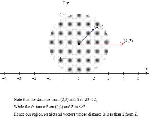
Let a = (1,2). Graph the open disc centered at a with radius 2.
  • An open disc centered at a with radius b is written as || x − a ||< b.
Recall that an open disc does not include its boundary, so that the graph of || x − (1,2) ||< 2 is
Let b = ( [1/2],[(√3 )/2] ). Verify that b is a unit vector.
  • A unit vector has its norm equal to 1, so we check that || b || = 1.
|| b || = √{( [1/2] )2 + ( [(√3 )/2] )2} = √{[1/4] + [3/4]} = √1 = 1.
Let a = ( √3 , − 2 ). Find the unit vector [(a)/(|| a ||)].
  • First we find the norm of a, so || a || = √{( √3 )2 + ( − 2)2} = √{3 + 4} = √7 .
  • Now we compute [(a)/(|| a ||)] = [(( √3 , − 2 ))/(√7 )] = [1/(√7 )]( √3 , − 2 ).
Our solution is ( √{[3/7]} , − [2/(√7 )] ). Note that this is a vector of lenght 1.
Let b = (1,0,2). Find a unit vector from b.
  • To convert b into a unit vector, we use the formula [(b)/(|| b ||)].
  • Computing the norm of b yields || b || = √{12 + 02 + 22} = √5 .
Our unit vector is [(1,0,2)/(√5 )] = ( [1/(√5 )],0,[2/(√5 )] ). We can verify this as || ( [1/(√5 )],0,[2/(√5 )] ) || = √{[1/5] + [4/5]} = 1.
Let u = (0,1) and v = (1,0).
i) Find || u + v ||2
  • Since u and v are perpendicular we can apply the pythagorean theorem for vectors so that || u + v ||2 = || u ||2 + || v ||2.
  • Since u and v are unit vectors, their norms are 1. That is || u ||2 = 1 and || v ||2 = 1.
Hence || u + v ||2 = || u ||2 + || v ||2 = 1 + 1 = 2.
Let u = (0,1) and v = (1,0).
ii) Find the angle q between u and v.
Since u and v are perpendicular we know that q = 90o.
Let a = ( − 2,5, − 1) and b = (4, − 3,1), find || a + b ||2.
  • Since a and b are not unit vectors, we compute the sume of the vectors first, followed by the norm.
  • a + b = ( − 2,5, − 1) + (4, − 3,1) = (2,2,0)
  • || a + b || = √{22 + 22 + 02} = 2√2
Our solution is || a + b ||2 = ( 2√2 )2 = 8. Note that from our previous step, || a + b ||2 = ( √{22 + 22 + 02} )2 = 22 + 22 + 02 = 8.
Find the angle θ between u = ( [1/(√2 )],[1/(√2 )] ) and v = ( [(√3 )/2], − [1/2] ).
  • The formula for finding the angle θ between two vectors is cosθ = [(u ×v)/(|| u |||| v ||)].
  • Note that both u and v are unit vectors, so that our equation is now cosθ = u ×v.
  • Computing the scalar product yields ( [1/(√2 )],[1/(√2 )] ) ×( [(√3 )/2], − [1/2] ) = [(√3 )/(2√2 )] − [1/(2√2 )] = [( − 1 + √3 )/(2√2 )].
The angle θ is then cos − 1( [( − 1 + √3 )/(2√2 )] ) = 75o.
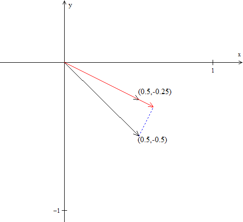
Find the projection from a to b given that a = ( [1/2], − [1/2] ) and b = ( [1/2], − [1/4] ).
  • Since a and b are not unit vectors, we use the general formula Pab = [(a ×b)/(b ×b)]b.
  • Computing we have, a ×b = ( [1/2], − [1/2] ) ×( [1/2], − [1/4] ) = [1/4] + [1/8] = [3/8]; b ×b = ( [1/2], − [1/4] ) ×( [1/2], − [1/4] ) = [1/4] + [1/16] = [5/16].
  • So that [(a ×b)/(b ×b)] = [(3 \mathord/ phantom 3 8 8)/(5 \mathord/ phantom 5 16 16)] = [6/5].
Hence Pab = [6/5]( [1/2], − [1/4] ) = ( [3/5], − [3/10] ). The image below displays how the projection (red vector) is perpendicular (blue line) to a but and extension of b.
Let w = ( [(a1)/(√3 )],0,[(a2)/(√3 )],0,[(a3)/(√3 )] ) where a12 + a22 + a32 = 3. Show that w is a unit vector.
  • We show that || w || = 1.
  • || w || = √{w ×w} = √{( [(a1)/(√3 )] )2 + 02 + ( [(a2)/(√3 )] )2 + 02 + ( [(a3)/(√3 )] )2} = √{[(a12 + a22 + a32)/3]} .
We can substitute the numerator with 3 so that || w || = √{[3/3]} = 1. So w is a unit vector.
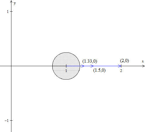
The sequence [1/n] is found when we replace n with the natural numbers 1,2,3, … Let a = (1,0).
i) Find the first five terms of the sequence 1 + [1/n].
  • By substituting n with 1,2,3,4 and 5 respectfully, we obtain the first five terms.
1 + [1/1] = 2, 1 + [1/2] = [3/2], 1 + [1/3] = [4/3], 1 + [1/4] = [5/4], and 1 + [1/5] = [6/5]. Note that the sequence is decreasing, never exceeding the previous term.
The sequence [1/n] is found when we replace n with the natural numbers 1,2,3, … Let a = (1,0).
ii) Is the sequence 1 + [1/n] contained in the closed disc centered at a with radius [1/4]? Explain.
Note that the first three terms are vectors of the form (2,0), ( [3/2],0 ) and ( [4/3],0 ) which are well outside the disc || x − (1,0) ||£[1/4]. Hence the sequence as a whole is not contained in the disc. See image.
The sequence [1/n] is found when we replace n with the natural numbers 1,2,3, … Let a = (1,0).
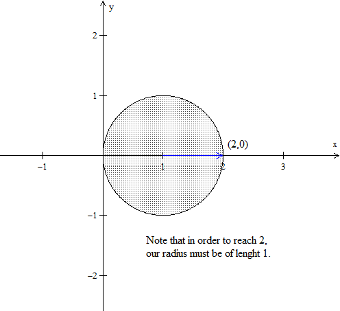
iii) What is the minimum radius b that will contain the sequence 1 + [1/n] in a closed disc? Explain.
  • Since our sequence is decreasing, we can see that as n reaches a high value, it will not exceed 1. For instance at n = 1000 we have [10001/1000] = 1.001
  • We base our radius b on the highest term available from the sequence, in this case 2.
Hence the disc discribed by || x − (1,0) || ≥ 1 is the minimum disc possible that will contain the entire sequence (as shown in the image).

*These practice questions are only helpful when you work on them offline on a piece of paper and then use the solution steps function to check your answer.

Answer

More on Vectors & Norms

Lecture Slides are screen-captured images of important points in the lecture. Students can download and print out these lecture slide images to do practice problems as well as take notes while watching the lecture.

  • Intro 0:00
  • More on Vectors and Norms 0:38
    • Open Disc
    • Close Disc
    • Open Ball, Closed Ball, and the Sphere
    • Property and Definition of Unit Vector
    • Example 1
    • Three Special Unit Vectors
    • General Pythagorean Theorem
    • Projection
    • Example 2
    • Example 3

Transcription: More on Vectors & Norms

Hello, and welcome back to educator.com.0000

Welcome back to multivariable Calculus.0003

Last lesson we introduced the scalar product, or dot product.0005

We also talked a little bit about norms.0008

Today, I am going to talk more about norms and vectors.0010

A lot of today, at least the first part of the lesson, is going to be basic properties.0015

Things that are pretty intuitively clear, but we want to formalize them.0020

Things that we are going to be talking about at any given moment.0024

We are going to be talking about open discs, open balls, and we want to make sure that we understand what these are, that we have been exposed to them so that we can proceed with our discussion of multivariable Calculus.0028

Okay, let us get started.0037

So let us let a be a point in the plane, remember a point is just a vector from the origin to that point.0040

A couple ways of thinking about it, let it be a point in the plane, let us see, then the set of points such that the norm, I should say the set of points x.0052

Let me do that.0084

It is the set of points x, such that the norm, in other words the distance between x and a, if it is less than some number, it is called the open disc.0085

Let me draw a picture of what this means.0105

Now, you know this notation here, so a norm is just a distance.0111

In the previous lesson, the norm between two points is the distance between those 2 points, that is all this is.0116

So this is saying that if there is a particular point in the plane, a, and if I want to take all of the points that are less than b units away from it -- let us say less than 2 units away from it -- I basically have all of the points in a circle, everything inside of that, here is what it looks like.0125

So here is our point a, let us go ahead and label that.0145

Then let us say b is some distance, b.0151

So all of the points in this disc, all of the points in here, all of the vectors, the points x such that the distance from x to , x to a, x to a, is less than sum b.0157

Basically it gives me a circular region in the plane that I am talking about.0173

Less than b, without this less than or equal to, we call it the open disc, so it is all of the points inside that circle of radius b.0181

It actually does not include all the points on the circle.0190

Now, if we say, the set of all points x such that the norm, in other words the distance from x to a,0193

Now if we say it is less than or equal to b, it is called the closed disc.0217

The closed disc actually includes, let me draw it separately up here, we have our a, then we have our b, it includes all points in here that are less than this length b.0227

But, it also includes all points on the boundary.0246

So closed, when we talk about an open set, we mean everything up to but not that boundary.0250

Closed is everything up to and including that boundary.0256

Now, let us see, this disc and a final one.0264

The set of all, actually I am not going to write it out since I have already written it out twice.0270

Let me just go ahead and give you the notation for it.0277

If we have the distance from the points x to a, which is the norm of x - a, if we say it equals b, well, this is the circle centered at a with radius b.0278

Now we are just talking about the boundary points, nothing outside, nothing inside.0300

So we have the open disc, we have the closed disc, and we have the circle.0305

We will often be talking about one of those or all of those.0310

It is very important that we specify which region in the plane we are talking about.0314

Now we are just going to generalize this, this is in 2 space.0318

Now we are going to generalize it to 3 space.0324

This is called the open disc, closed disc, the circle, we call it the... so for n=3, well let us say, for R3, let us be consistent, we have the closed ball and the sphere.0326

It is the same notation, the set of all x, either less than b, or less than or equal to b, or equal to b.0358

In 3 dimensions, we basically have that the picture we have is this.0373

Just do a quick picture of it, some point, and then instead of a circle, what you have is a ball.0377

That is it, just a ball, you have some center, you know this center right here is the point a, the vector a.0388

Then the radius of this ball is b.0396

So that is all it is.0401

This nomenclature of ball, closed ball, that actually applies to any number of dimensions.0404

So if I want to talk about the open ball in the 5th dimension, that is what it is.0412

It tells me there is some vector a in the center, and then all the points that are less than some specified value away from that point, we call it the open ball, the closed ball, the open sphere, depending on which set of points we are talking about.0415

Alright, let us move on.0435

We are just talking about things that we are going to be using over and over again.0436

So this is going to be a property, again this particular property is intuitive, but we might as well formalize it.0440

Let x be a number, then the norm of x × a, a vector, = x × norm of a.0450

What this says is that if I have a vector a and I multiply it by some number, let us say 15, then I take the norm of what I get.0470

It is the same as taking the norm of the vector first, and then multiplying by the number 15 afterward.0480

This is intuitively clear, but then I will formalize it.0485

Okay, now, let us give a definition.0489

Now I am going to define something called a unit vector.0496

It is exactly what you think it is, a unit vector is a vector whose norm is one.0498

In other words, whose length is 1.0507

Formally, that is, if the norm is 1, it is a unit vector.0513

That is it, it is just a unit vector whose length is 1.0520

1 is nice because it is one of those numbers that you can use as a standard and you can multiply it by any number you want to make it as big as you want, or to make it as small as you want.0523

In mathematics it is called the identity, in mathematics it is a very important number.0535

Okay, given any vector, b, just a random vector -- let me do this notation a little differently.0537

1/norm(b), and the norm is a number, × the vector b itself = a unit vector in the direction of b.0555

This is very important, so basically if I am given some vector b of any specified length, I can actually take that vector.0576

And, if I divide that vector by its norm, or more specifically, if I multiply it by the reciprocal of its norm as a constant in the front, remember we can do that, we can multiply vectors by constants, lengthen them, shorten them -- I can actually create a unit vector, specifically a vector of length 1 in the direction b.0586

That is what makes this very nice.0609

You have any vector, you just go ahead and you essentially divide it by its norm, and you have created a unit vector.0611

That is standard procedure for creating a unit vector in any given direction.0616

It is going to be very important when we talk about the direction of derivatives later on.0621

Now a little bit more, we say 2 vectors have the same direction.0630

Let me see, let me specify what they are, actually.0645

We say that 2 vectors a and b, have the same direction if there is some number C, such that C × a = b, or a = c ×b,0653

Where you put the c does not matter.0685

All that says if I have 2 vectors, let us say that, and that, I can find some number since they are in the same direction.0687

Basically we know that when you multiply a vector by a scalar, by some number, all you do is you lengthen it or shorten it, you scale it out.0695

You are scaling it, that is where the word scalar comes from.0702

If this is a, and this is b, well I know that if I start with a and it looks like here I maybe have to multiply it by 3 to get b.0706

If there is such a number that I can multiply by a to get b, that automatically tells me that a and b are in the same direction.0717

I do not necessarily know that, but this property allows me to say the two vectors happen to be in the same direction.0724

If I need to check they are in the same direction, I need to find some number c that satisfies this property.0732

Let us say I start with some vector b and I need to see if a happens to be in the same direction,0737

If I can take b and multiply it by 1/3, I can get a, sure enough there is some number b that if I multiply by 1/3, I end up getting the vector a.0745

That means they are in the same direction.0755

So this is just a formal definition of when some things are in the same direction.0757

Again, what mathematics does, it takes things that are generally intuitive and it actually formalizes them.0763

It gives them specific algebraic definitions so that we can actually do something with them.0770

Geometry helps, we want to be able to draw a picture and talk about two vectors in the same direction.0775

But geometry is not math, geometry is just some sort of pictorial representation that helps you visualize something.0780

It is algebra that is math, that is where the power of mathematics comes in.0787

Now, let us move on with some more unit vectors.0795

Unit vectors are fantastic because we can basically take any vector and we can convert it to a unit vector.0799

Once we convert it to a unit vector, then we can multiply that unit vector by any number c to make it any length that we want.0807

That is the power of unit vectors, it gives us a standard, an identity vector, if you will,0814

To multiply by, that we can always use over and over again.0822

I can get any length I want by just choosing the proper c.0825

If I have a unit vector and I want a length of 15, I can just multiply it by 15.0829

If I want it to be a vector in the opposite direction to have a length of 446, I take -446 × my unit vector.0833

Let us do an example.0845

Okay, so example number 1.0850

Let the vector a = (3,2,-1), so we are working in R3, 3 dimensional space.0855

Now the norm, let us go ahead and calculate the norm, we are going to be finding the unit vector in this direction.0863

Again, we need to find the norm so that we can actually multiply by the reciprocal of the norm or divide by the norm to create the unit vector.0870

So, the norm of a, you remember from Calculus that things started to get a little notationally intensive.0878

In multivariable calculus, things are going to get even more notationally intensive.0888

Do not let the tedium of the notation throw you off, it is just notation.0890

You want to be very, very clear about what you are doing.0894

Whatever you do, do not do things in your head, write out everything.0897

This is very important.0900

When you are doing things in your head, I think it is really nice to be able to do that.0903

But the idea in mathematics is to be correct, to know what is going on, not to show somebody that you can do something in your head.0908

If you write things out, especially because this is not arithmetic anymore, this is serious upper level math, this is real mathematics.0913

You want to be able to notate everything properly.0924

I know it is tedious, but write out the notation, it equals sqrt(9) + 4 + 1, and we end up with sqrt(14).0927

So, the unit vector in the direction of a which I will symbolize like that.0945

We are often going to be throwing symbols in here that are a little less than standard, that you may not see in your book.0952

I will certainly try to be as standard as possible, I will try to use notation that you will see all the time.0960

But again, a lot of times when we are talking about a concept, we need to be able to use notations that make sense at the moment.0965

You are free to do that yourself.0972

What is important is not the symbolism, but the underlying mathematics.0975

This is just a symbol for a unit vector in the direction of a, you can symbolize it any way you want.0977

= 1/sqrt(14) × the vector (3,2,-1).0984

Right? Because we said a unit vector is just 1/reciprocal of the norm × the vector itself.0993

Well the vector is this.1001

When we multiply a constant by a vector, we multiply everything by that constant,1005

So we get 3/sqrt(14), 2/sqrt(14) and -1/(sqrt14), this is a perfectly good vector, you can leave it like that.1009

You do not need to rationalize the denominator like they made you do in high school.1020

It is a perfectly valid number, it is a unit vector in the direction of a.1025

If you were to take the norm of this number, you would find that its norm is 1, you have created a unit vector.1033

You might want to do that yourself just to convince yourself that this is true.1039

Okay, now we are going to talk about 3 very special unit vectors.1044

So, 3 special unit vectors.1050

And we are going to be talking about our 3 dimensional space, so we have the z axis, the x-axis, and the y-axis.1060

Let me go ahead and label those.1069

Again, this is the standard right handed representation of three dimensional space, x, y, z.1074

Well, a vector in the direction of z, a vector in the direction of x, and a vector in the direction of y -- each having a length of 1 -- each of those have special names.1080

We call them, we can go ahead and say e1, or we can go ahead and say, you know what, I am going to use ex.1096

So this vector right here, the point, remember, it is a point that a unit vector represents, is (1,0,0).1106

My notation is not doing too well today, my apologies, (1,0,0), that is it.1125

Now the unit vector in the direction of y is notated as ey, sometimes notated as e2.1130

It equals (0,1,0), there is nothing in the x direction, nothing in the z direction, but a length of 1 in the y direction.1139

Of course ez is equal to (0,0,1).1150

These are mutually perpendicular, they are orthogonal.1155

In other words if you took the dot product of this, it would be 0, this and this, 0, this and this, 0.1157

That is the whole idea.1163

This is called an ortho-normal-basis, you do not have to know that.1164

Just know that they are perpendicular.1168

Because we often talk about 3 space, we will often be using 3 space and 2 space.1171

We just wanted to introduce this special collection of unit vectors in the direction of the coordinate axes.1176

Okay, now let us go ahead and do our general Pythagorean theorem.1184

You know our Pythagorean theorem, it is of course if you have a right triangle in the plane, a2 + b2 = c2.1188

The sum of the squares of the two shorter sides is equal to the square of the hypotenuse.1197

As it turns out this is generally true in all dimensions.1200

I am not going to go ahead and do a proof of the theorem.1205

Again, in these set of courses, we want to be able to list the theorems, and we want to be able to use them, but we are not going to go through the proofs.1207

We want to do it in an intuitive sense, we want to get a feeling of it by doing problems and by discussing it, not necessarily by doing proofs.1218

If you want the proofs, by all means they are in your book.1225

I would certainly suggest looking at them at least occasionally.1228

At least to see what is going on if something seems like it fell out of the sky.1230

Most of these things are reasonably intuitively clear.1232

The general Pythagorean Theorem, we are going to be using norm notation, so again a norm is a length -- if a and b are orthogonal, in other words if their dot product is equal to 0, if they are perpendicular, then the norm of a + b 2 = norm(a2) + norm(b2).1237

Again, a norm is a length.1282

It tells me that if I have a and b that are orthogonal to each other, a and b orthogonal to each other, the length of a2 + the length of b2 is equal to the length of a+b2.1284

That is that length, that is all that is going on, this is just the standard Pythagorean theorem expressed for any number of dimensions.1300

You can have R3, R5, R15, it does not matter.1308

It holds in all dimensions, that is actually pretty extraordinary that it does so.1312

Let me go ahead and draw this out a little bit more formally here.1319

If this is a and this is b, well, so this is vector a and this is the vector b, the vector a+b is this vector.1325

Remember when we said if we add vectors, we go from tail to head of one, then we take b, that direction, and we just go this way.1335

That is it, this is a + b, you start here and end up here, then you start here and you end up here.1347

So this vector right here actually is a+b.1351

Of course this is perpendicular therefore this is perpendicular, so this vector here is our a+b.1360

Sure enough, this squared + this squared = that squared, that is all this is saying.1368

The norm of this + the norm of that = the norm of this.1372

Now we are going to introduce a very very important notion, something called a projection and we will do an example of that.1380

A projection, let us go ahead and define what we mean by that.1390

First of all I am going to draw a picture.1392

Let us say I have a vector a, and another vector b, so this is a and this is b, the order is very important here.1400

If I imagine shining a light straight down this way, this a is actually going to cast a shadow on this vector b.1410

That shadow is of course, if you shine the light straight down, it is going to be perpendicular to that.1421

This thing right here, this vector, it is a vector along b, but its length is the actual length of the shadow that is cast by the vector a.1427

Obviously if this angle were bigger, then you would have a shorter shadow.1442

This thing right here, that is the projection.1447

It is the projection of a onto b.1450

I am going to notate it this way.1455

The projection is an actual vector.1457

The projection of a onto b.1460

This is going to be the notation that I use for my projection, it is a slightly different than you are going to use in your book but I think it makes everything clear.1464

You are saying that you are projecting the vector a onto the vector b, not the vector b onto the vector a.1472

That actually exists, you can project any vector onto another vector, but it is an entirely different vector.1480

The order matters.1484

The algebraic definition of the projection, this is the geometric, we just wanted to see what we mean by that in 2 space and 3 space, so algebraically, the project of a onto b = a · b/b · b ×, so this is a number, × the vector b itself.1487

a · b/b · b is just some number, so basically what we are doing is, again, we want to find what this vector is.1518

It is in the direction of b, so we know that this vector is some number × b, right?1528

It is basically just you are scaling out b, you either make it bigger or smaller, in this case it ends up being smaller.1535

That is all you are doing, is we want to know what vector = the projection of this vector on top of this vector.1545

The projection geometrically is what shadow does this cast on that.1554

Again, this is just some number, dot products are just numbers.1560

A number × a number, we are scaling b to find out what this is.1564

Now, let us move on to the next set.1570

The component of a along b, let me actually, so c = a · b/ b · b, all this is is just the component of the vector a along the vector b.1576

In other words, if I take a look at this vector a, it has this component this way, and another component this way.1605

It is the component of a in the direction of b, that is all it is.1613

The best way to think about it is this whole idea of shining a light and casting a shadow, that is what is going on.1618

If b happens to be a unit vector, then since the norm of b = 1, b · b, that denominator = 1.1628

Remember the definition of the norm is the square root of the dot product.1657

So if the norm is 1, and I take the square of that which is also 1, it means that that product is 1.1661

The projection of a onto b = just a · b × vector b.1672

In other words the denominator disappears, because b · b = 1.1683

So if you happen to be projecting something onto a unit vector, which looks like this, let us say that is a vector of unit 1 and this is b.1685

It is not a unit vector of 1, it is a unit vector, so it has a length of 1, my apologies.1697

If that is a, well again, if I shine a light, drop a perpendicular, that is all I get.1701

I drop a perpendicular from the end of a down onto the vector b, well, the vector b extends this way, right?1708

But this is a unit vector, so what I am looking for is that vector.1717

It has a length and it has a direction.1720

That length and that direction is given by this expression right here, if b happens to be a unit vector.1723

If not, then you just use a general vector addition.1730

So let us do an example.1735

Example number 2.1740

We will let a = (2,4,2) and b = (-3,1,3).1743

Okay, now we want to find the projection of a onto b.1755

Well we use our formula, so the projection of a onto b = a · b/ b · b × vector b itself.1763

Okay, well, a · b = 2 × -3 is -6, 4 × 1 is 4, 2 ×3 is 6, -6 + 6 is 0, so that is 4.1783

And b · b = -3 × 3 is 9, and 1 × 1 is 1, and 3 × 3 is 9, so we get 19, if I am not mistaken.1799

Therefore the projection equals 4/19 × vector b itself.1814

Well the vector b is, I am going to write it vertically, (-3,1,3).1823

Of course we have a constant times a vector, so we multiply everything right through.1834

So that is (-12/19, 4/19, 12/19), this vector (-12/19, 4/19,12/19) it is the projection of the vector (2,4,2) on (-3,1,3) in that direction.1838

That is what is going on here.1863

That is it, this is algebraic.1865

Very, very important.1868

Let us go ahead and finish it off with a nice further geometric interpretation, so let us go ahead and take our standard drawing of, this is vector a and this is vector b, and we know that this is the projection right perpendicular.1873

So this right here happens to be, this length is the norm(a), that is what the length is, what the norm is, it is a length.1890

This length right here, well it happens to be, remember c × the norm(b).1900

Basically I have taken the length of b and I have multiplied by some number c, and that c = that a · b/b · b.1908

This would be our definition.1920

So if I have the norm of b, and I multiply by this a · b / b · b, from the projection, that is the length of this thing.1923

If I, now look, I have some angle θ in between those 2 vectors, in between this vector and this vector or this vector and this vector, it actually does not really matter.1934

I can actually write cos(θ) = the adjacent/the hypotenuse of this right triangle.1945

So I end up with c × norm(b)/the norm(a).1950

C happens to be a · b/b · b, and I am multiplying that by the norm(b).1960

Then I divide all of that by the norm(a).1978

Remember the definition of the norm, remember the norm(b), or any vector, is the sqrt(b · b).1983

So b · b, if I square both sides, I get the norm squared.1997

So I am going to take b · b, and I am going to replace this with that.2004

So that equals a · b/the norm of b2 × the norm divided by the norm of a.2010

Okay, now this is squared, this is on top, this cancels this, and of course when I rearrange this because this is actually equal to a · b/norm of b × norm of a.2027

Look at that.2045

I have the cosine of the angle θ between those two vectors = the dot product of those vectors/the product of the norms of those vectors.2048

Or, another way of writing it is a · b = norm(a) × norm(b) × cos(θ).2063

In some books, possibly in your own, this is actually taken to be the definition of the dot product.2079

That is fine, it is not really a problem in and of itself.2085

However, notice we have introduced some angle θ.2093

Well the angle θ makes sense in 2 and 3 dimensions.2096

The algebraic definition of dot product which we gave is the product of the, you know, corresponding entries added together.2100

That strictly involves a and b, it does not involve something else, and it does not involve something else called the norm.2111

I think this is fine, I think it is better to use the algebraic definition and derive this as an identity as opposed to taking this as a definition.2120

The nice thing about it is all of the other properties of the scalar product fall out easily when you use the algebraic definition as opposed to this definition.2129

Starting out with this definition, it is okay, but I think it is just better mathematically to work the other way around.2138

Notice we had just a nice straight basic definition of the dot product, and then we ended up with this identity.2149

Let us go ahead and do our final example for this lesson.2155

Example 3.2162

We will let a = (2,-2,6) and we will let b = (3,0,1).2165

We want to find θ, the angle between those vectors.2175

Well, we know that cos(θ) = a · b/norm(a) × norm(b).2190

a · b = 6 + 0 + 6,2205

The norm of a, if I do that out is going to be sqrt(44).2211

The norm(b) is going to be sqrt(10).2215

I end up with 12/sqrt(440), which is equal to 0.5721.2218

When I take the inverse cos, or arccos, I get θ = 55.1 degrees.2228

That is it, so you have 2 vectors in 3 space, the angle between them is 55.1 degrees.2240

We used the norm, and we used the dot product.2245

It is fine to think about this geometrically when you think about our angle in R2, or an angle in R3.2250

We do not really talk about angles in R4 or R5, they do not really make sense.2257

We can still certainly talk about them, this value still exists, this identity is still valid, but again, we would like to make sure that we work algebraically, not just geometrically.2260

Do not try to figure intuition and make it fit the mathematics, do not try to make the mathematics fit your intuition.2275

Let the mathematics guide you.2283

At the end you have to defer to the mathematics, not your intuition.2288

Now that we are getting into higher mathematics your intuition will not always lead you in the right direction.2291

Thank you for joining us here at educator.com, we will see you next time.2295

Educator®

Please sign in to participate in this lecture discussion.

Resetting Your Password?
OR

Start Learning Now

Our free lessons will get you started (Adobe Flash® required).
Get immediate access to our entire library.

Membership Overview

  • Available 24/7. Unlimited Access to Our Entire Library.
  • Search and jump to exactly what you want to learn.
  • *Ask questions and get answers from the community and our teachers!
  • Practice questions with step-by-step solutions.
  • Download lecture slides for taking notes.
  • Track your course viewing progress.
  • Accessible anytime, anywhere with our Android and iOS apps.